
Transformer Step2 Modern LLM
nanoGPT의 vanilla Decoder-only Transformer에서 출발해 LLaMA의 block 현대화, SWA·FlashAttention, KV Cache, MHA→MQA→GQA→MLA, Mixtral MoE, 그리고 serving 기술까지 하나의 흐름으로 정리한다.
목적: nanoGPT에서 배운 vanilla Decoder-only Transformer를 출발점으로, 현대 LLM에서 반복적으로 등장하는 block 구조 + long-context/attention 효율화 + KV memory + MoE + inference system 개념을 하나의 흐름으로 이해한다.
이 페이지의 핵심 질문
- Transformer block 자체는 무엇이 바뀌었는가?
- Context가 길어지면 왜 Attention과 KV Cache가 병목이 되는가?
- FlashAttention / SWA / GQA / MLA는 각각 무엇을 줄이는가?
- MoE는 왜 parameter를 크게 늘리면서도 token당 계산량을 제한할 수 있는가?
- 실제 serving에서는 PagedAttention, batching, quantization, speculative decoding이 왜 필요한가?
Contents
- Modern Transformer Block — LLaMA
- RMSNorm / Pre-Norm
- RoPE
- SwiGLU
- LLaMA: Open and Efficient Foundation Language Models
- Long Context & Attention Efficiency
- Full causal attention
- Sliding Window Attention
- FlashAttention
- Mistral 7B
- FlashAttention
- KV Cache — Autoregressive Inference의 핵심
- Prefill vs Decode
- 왜 Q는 cache하지 않고 K,V만 cache하는가
- KV Cache memory가 왜 커지는가
- MHA → MQA → GQA → MLA
- KV head 공유
- KV Cache 감소
- DeepSeek의 latent compression
- Fast Transformer Decoding: One Write-Head is All You Need
- GQA: Training Generalized Multi-Query Transformer Models from Multi-Head Checkpoints
- DeepSeek-V2
- MoE — Mixtral
- Dense FFN → Router + Experts
- Top-k routing
- Active params vs Total params
- Load balancing / communication
- Mixtral of Experts
- Modern Inference Techniques
- PagedAttention
- Continuous Batching
- Quantization
- Speculative Decoding
- vLLM / PagedAttention
- Fast Inference from Transformers via Speculative Decoding
- 2026 관점에서 보는 Architecture Branch
- GQA 계열
- MLA 계열
- MoE 계열
- Long-context / local-global attention 계열
0. 먼저 전체 그림
1
2
3
4
5
6
7
8
9
10
11
12
13
14
15
16
17
18
19
20
21
22
23
24
25
26
27
28
29
30
nanoGPT
Vanilla Decoder-only Transformer
        │
        ▼
LLaMA
"Transformer block 자체를 현대화"
RMSNorm + RoPE + SwiGLU
        │
        ▼
Context / inference bottleneck
Attention cost 증가
KV Cache 증가
        │
        ├── FlashAttention
        │      Attention 계산의 memory I/O 효율화
        │
        ├── SWA / Local Attention
        │      직접 보는 token 수 감소
        │
        └── MQA / GQA / MLA
               저장할 KV 자체를 감소
        │
        ▼
MoE
Dense FFN 전체를 매번 계산하지 말자
        │
        ▼
Serving / Inference System
PagedAttention + Continuous Batching
+ Quantization + Speculative Decoding
핵심: FlashAttention, KV Cache, GQA는 같은 기술이 아니다.
- FlashAttention = Attention 계산 자체를 GPU memory-efficient하게 수행
- KV Cache = autoregressive decoding에서 과거 K,V를 다시 계산하지 않도록 저장
- MQA / GQA / MLA = 저장해야 하는 K,V의 양 자체를 줄임
- SWA = 한 token이 직접 보는 context 범위를 줄임
1. LLaMA — Modern Transformer Block
LLaMA는 완전히 새로운 종류의 Transformer를 만든 것이 아니다. nanoGPT에서 배운 Decoder-only Transformer 골격을 유지하면서 각 block의 핵심 부품을 현대화했다.
1
2
3
4
Token embedding
  → [RMSNorm → Causal Self-Attention → Residual
     RMSNorm → SwiGLU FFN           → Residual] × N
  → Final RMSNorm → LM Head → next-token logits
1.1 Training Data
- English Common Crawl
- C4
- Github
- Wikipedia
- Gutenberg and Books
- ArXiv
- Stack Exchange
Tokenizer는 BPE(Byte-Pair Encoding) 계열을 사용한다.
1.2 RMSNorm + Pre-Norm
LayerNorm은 평균을 빼고 분산으로 나눈다. 반면 RMSNorm은 centering을 생략하고 vector의 RMS 크기를 이용해 rescale한다.
1
2
LayerNorm: 평균을 0으로 맞춤 + 크기를 정규화
RMSNorm:                 크기만 정규화
LLaMA는 RMSNorm을 Pre-Norm으로 사용한다. 즉 Attention/FFN을 통과한 뒤가 아니라 sub-layer에 들어가기 직전 normalization을 적용한다.
위치: Attention 앞, FFN 앞
1.3 RoPE — position은 어디에 들어가는가?
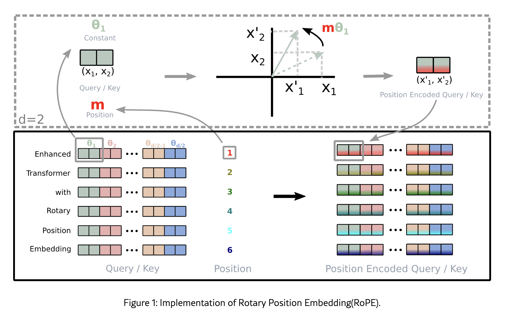
Absolute Position Embedding은 token embedding에 위치 vector를 더한다. 반면 RoPE (Rotary Positional Embedding)는 Attention 내부에서 position에 따라 Q와 K vector를 회전시킨다.
1
2
기존: token embedding + position embedding → Q, K, V
RoPE: token embedding → Q, K, V → position에 따라 Q와 K 회전
회전된 Q와 K의 dot product에는 두 token의 상대적인 위치 관계가 자연스럽게 반영된다.
위치: Self-Attention 내부, Q/K projection 이후, attention score 계산 이전
1.4 SwiGLU — FFN은 어떻게 바뀌었는가?
nanoGPT의 단순 FFN을 생각하면 대략 Linear → activation → Linear 구조다. LLaMA는 이를 SwiGLU FFN으로 교체한다.
1
2
3
4
일반 FFN:  x → Up Linear → activation → Down Linear

SwiGLU:    x → Gate Linear → SiLU ─┐
             → Up Linear ──────────× → Down Linear
gate branch가 token마다 어떤 feature를 얼마나 통과시킬지를 조절한다. 뒤에서 볼 Mixtral의 Expert 하나도 결국 서로 다른 weight를 가진 SwiGLU FFN 하나다.
2. Long Context & Attention Efficiency
2.1 Vanilla Full Causal Attention
현재 token i는 자신보다 앞에 있는 모든 token 0…i를 볼 수 있다.
1
token i → [0, 1, 2, ... , i]
Sequence 길이를 N이라 하면 training/prefill에서 attention score matrix는 대략 N × N이므로 계산량이 빠르게 증가한다. 문제는 두 종류다.
- Attention 계산 자체가 비싸진다.
- Inference에서는 과거 token들의 K,V를 계속 저장해야 한다.
이 둘은 관련되어 있지만 서로 다른 병목이다.
2.2 Sliding Window Attention (SWA)
Mistral 7B는 현재 token이 직접 보는 범위를 최근 W개로 제한한다.
1
2
Full Attention: token i → [0, 1, 2, …, i]
SWA:            token i → [i-W, …, i]
직접 Attention 범위가 짧아져 계산량을 줄일 수 있다. 여러 layer가 쌓이면 hidden state를 통해 더 먼 정보가 간접적으로 전달된다.
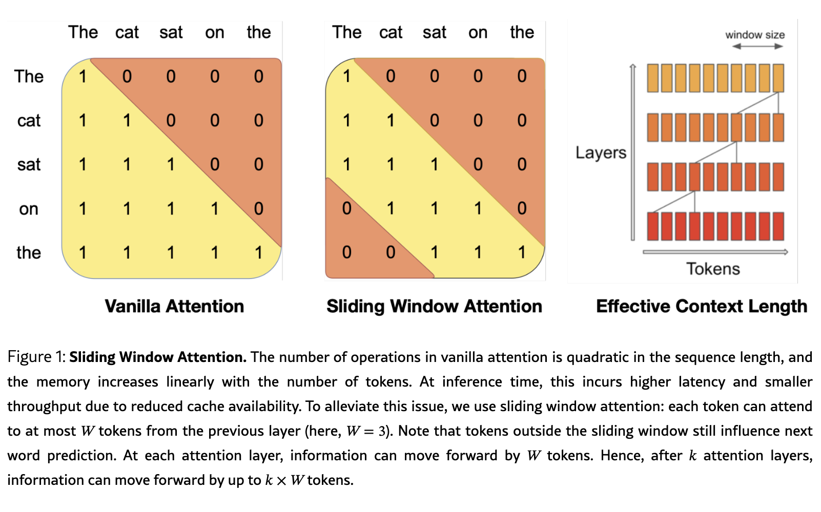
SWA가 줄이는 것: 한 layer에서 직접 비교하는 token 수
원문: Mistral 7B §2 Architectural details
2.3 FlashAttention — 같은 Attention을 더 효율적으로 계산
FlashAttention은 attention pattern을 바꾸는 방법이 아니다.
1
QKᵀ → softmax → V
라는 수학 자체는 그대로 유지하면서, GPU의 HBM과 on-chip SRAM 사이의 data movement를 줄이는 방식으로 attention을 tile 단위로 계산한다. 따라서 Full Attention을 FlashAttention으로 계산해도 여전히 이론적인 attention pair 수 자체는 full attention이다.
FlashAttention이 줄이는 것: Attention 계산 과정의 memory I/O와 materialization overhead
논문: FlashAttention: Fast and Memory-Efficient Exact Attention with IO-Awareness
SWA vs FlashAttention
| 기술 | 바꾸는 것 | 핵심 목적 |
|---|---|---|
| Full Attention | 모든 과거 token을 직접 봄 | 최대 context connectivity |
| SWA | 보는 token 범위를 줄임 | Attention pair 자체 감소 |
| FlashAttention | 계산 순서/메모리 접근을 최적화 | 같은 attention을 GPU에서 효율적으로 계산 |
3. KV Cache — Autoregressive Inference의 핵심
3.1 왜 KV Cache가 필요한가?
LLM inference는 한 번에 문장 전체를 생성하지 않는다.
1
2
3
4
Prompt → token 1 생성
       → token 2 생성
       → token 3 생성
       → ...
새 token을 생성할 때마다 이전 token들의 K,V는 변하지 않는다.
1
2
3
4
5
6
7
8
9
10
token 1 생성
→ K1, V1 계산

token 2 생성
→ K1,V1 재사용
→ K2,V2만 새로 계산

token 3 생성
→ K1,V1,K2,V2 재사용
→ K3,V3만 새로 계산
이전 K,V를 저장해 두는 것이 KV Cache다. KV Cache가 없다면 매 token 생성마다 과거 sequence 전체의 K,V를 다시 계산해야 한다.
3.2 왜 Q는 Cache하지 않는가?
현재 step에서 필요한 Query는 지금 생성 중인 token의 Q다.
1
2
3
4
5
6
7
현재 Q_t
   ↓
[과거 K_1 ... K_t]와 dot product
   ↓
attention weights
   ↓
[과거 V_1 ... V_t] weighted sum
과거 token의 Q는 다음 token 생성 시 다시 사용할 필요가 없다. 반면 K,V는 미래 token들이 계속 참조한다.
그래서 이름이 KV Cache이고 Q Cache가 아니다.
3.3 Prefill vs Decode
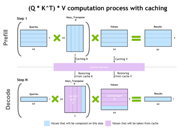
Autoregressive inference를 이해할 때 이 구분이 매우 중요하다.
Prefill
Prompt 전체를 한 번에 넣어 각 token의 hidden state와 K,V를 계산한다.
1
2
3
4
5
Prompt: [A B C D E]
       ↓
A~E 전체를 parallel하게 처리
       ↓
KV Cache 생성
Prefill은 sequence가 길수록 Attention 계산량의 영향을 크게 받는다.
Decode
그 다음부터는 token을 하나씩 생성한다.
1
2
3
4
step 1: Q_new × cached K
step 2: Q_new × cached K
step 3: Q_new × cached K
...
Decode에서는 matrix 연산 크기가 작고, 대신 저장된 KV를 계속 읽어야 하기 때문에 memory bandwidth / KV Cache가 매우 중요해진다.
매우 단순화하면:
- Prefill: compute-heavy
- Decode: memory-bandwidth-heavy
3.4 KV Cache가 왜 병목이 되는가?
KV Cache 크기는 대략 다음 요소에 비례한다.
1
2
3
4
5
6
7
8
KV memory
∝ batch size
× sequence length
× number of layers
× number of KV heads
× head dimension
× 2 (K + V)
× bytes per element
따라서 context가 길어지고 batch가 커질수록 GPU memory를 빠르게 차지한다. 그리고 여기서 자연스럽게 다음 질문이 나온다.
“모든 Query head마다 K,V head를 따로 저장할 필요가 있는가?”
이 질문이 MHA → MQA → GQA → MLA로 연결된다.
4. MHA → MQA → GQA → MLA
4.1 Multi-Head Attention (MHA)
기본 MHA에서는 Q,K,V 모두 여러 head를 가진다.
1
2
3
Q: q1 q2 q3 q4 q5 q6 q7 q8
K: k1 k2 k3 k4 k5 k6 k7 k8
V: v1 v2 v3 v4 v5 v6 v7 v8
표현력은 좋지만 inference에서는 모든 K,V head를 저장해야 한다.
4.2 Multi-Query Attention (MQA)
MQA는 여러 Query head가 하나의 K/V head를 공유한다.
1
2
3
4
Q: q1 q2 q3 q4 q5 q6 q7 q8
             │
K:           k1
V:           v1
KV Cache와 memory bandwidth를 크게 줄일 수 있지만, K/V 표현 capacity를 너무 많이 줄일 수 있다.
논문: Fast Transformer Decoding: One Write-Head is All You Need
4.3 Grouped-Query Attention (GQA)
GQA는 MHA와 MQA의 중간이다. 여러 Query head를 group으로 묶고 각 group이 하나의 K/V head를 공유한다.
1
2
3
4
Q: q1 q2 | q3 q4 | q5 q6 | q7 q8
     │       │       │       │
K:  k1      k2      k3      k4
V:  v1      v2      v3      v4
Mistral 7B도 GQA를 사용한다.
SWA = 얼마나 먼 token을 볼 것인가?
GQA = 몇 개의 K/V head를 저장할 것인가?
Reference: GQA: Training Generalized Multi-Query Transformer Models from Multi-Head Checkpoints
4.4 MLA — Multi-head Latent Attention
💡 DeepSeek 계열에서 중요한 아이디어는 KV 자체를 더 작은 latent representation으로 압축해 저장하는 것이다.
매우 단순화하면:
1
2
3
4
5
6
7
8
9
10
11
MHA/GQA
hidden state
  → K heads
  → V heads
  → KV Cache에 직접 저장

MLA
hidden state
  → low-dimensional latent c
  → cache에는 c 중심으로 저장
  → 필요할 때 K/V representation을 복원/사용
즉 GQA가 KV head 수를 줄이는 방법이라면, MLA는 KV 정보를 low-rank latent space로 압축하는 방법에 가깝다.
MLA를 이해할 때 핵심은 “Attention을 완전히 다른 것으로 바꿨다”보다 KV Cache compression을 architecture 수준에서 설계했다는 점이다.
출처: DeepSeek-V2: A Strong, Economical, and Efficient Mixture-of-Experts Language Model, DeepSeek-V3 Technical Report
MHA / MQA / GQA / MLA 한 번에 비교
| 방식 | Q heads | KV 구조 | 핵심 효과 |
|---|---|---|---|
| MHA | 많음 | Q head마다 K,V | 최대 표현력, KV 큼 |
| MQA | 많음 | K,V 1개 공유 | KV 매우 작음 |
| GQA | 많음 | group별 K,V | 표현력/메모리 절충 |
| MLA | 많음 | latent representation으로 압축 | KV memory를 구조적으로 감소 |
5. Mixtral — Mixture of Experts (MoE)
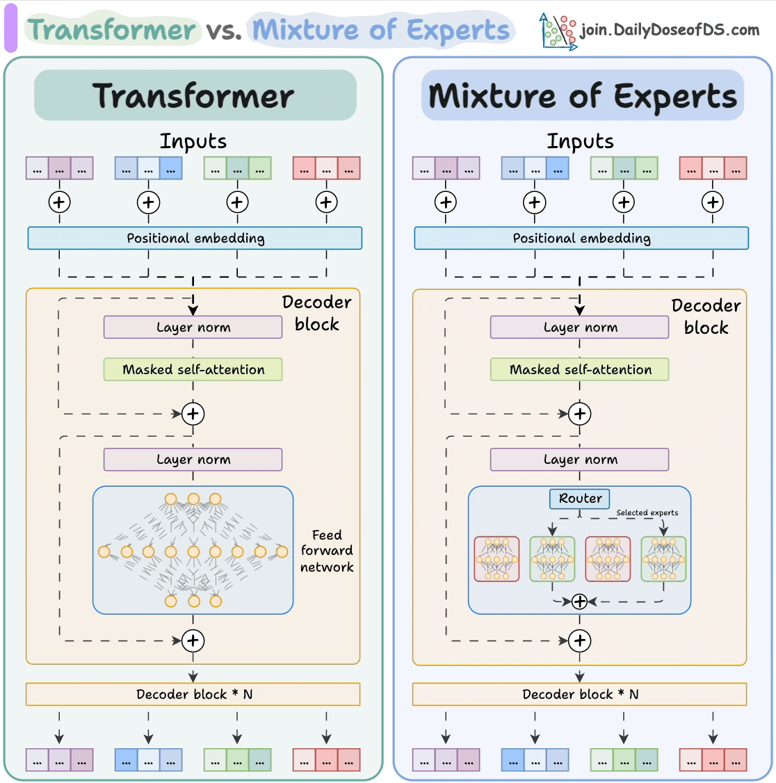
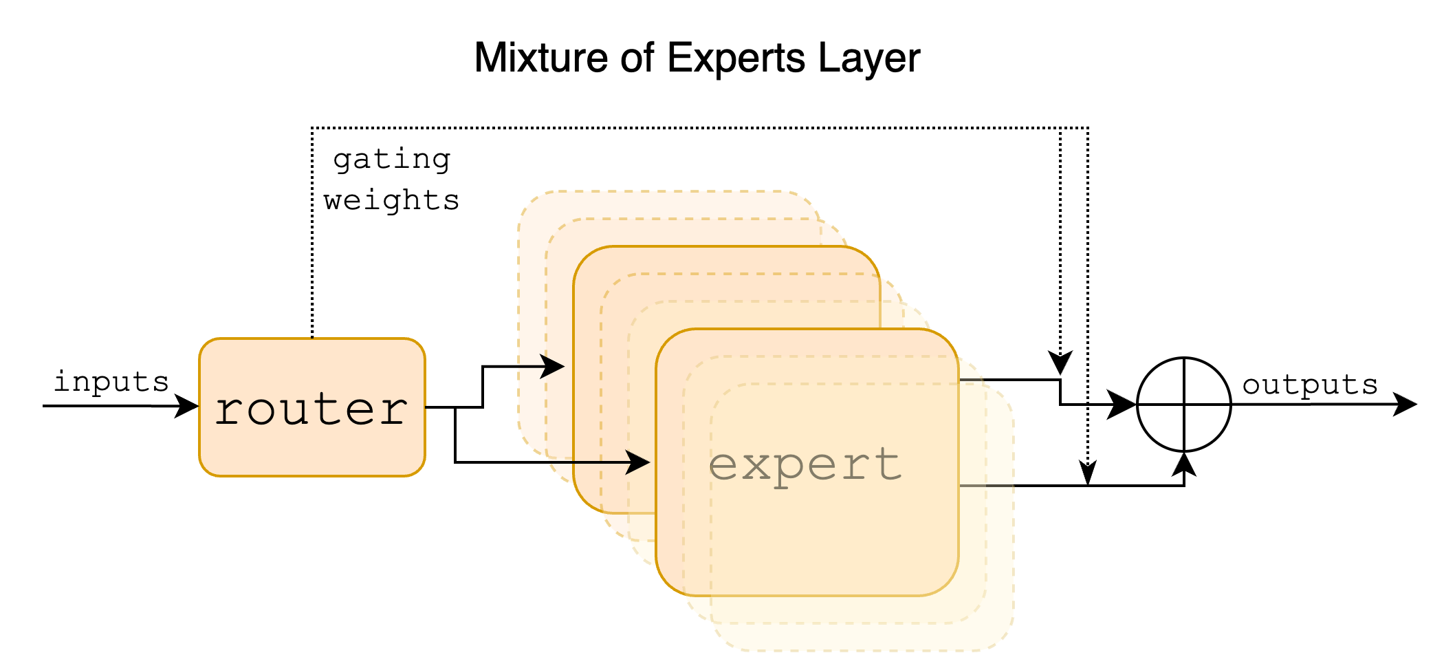
MoE는 Attention을 바꾸는 것이 아니다. Transformer block의 FFN 부분을 sparse expert 구조로 교체하는 것이다.
1
2
3
4
5
6
7
8
9
10
11
12
13
14
15
16
17
18
19
20
21
22
23
24
25
입력 hidden state x
       │
       ▼
   RMSNorm
       │
       ▼
Self-Attention
       │
       ▼
Residual Add
       │
       ▼
   RMSNorm
       │
       ▼
Router Linear → Top-k routing
       │
       ├── Expert 1: SwiGLU FFN ─┐
       ├── Expert 2: SwiGLU FFN ─┤ 선택된 expert만 계산
       └── Expert 3…N: 계산 안 함 │
                                 ▼
                          weighted sum
                                 │
                                 ▼
                           Residual Add
5.1 Expert 하나는 무엇인가?
Expert 하나는 별도의 Transformer나 Attention head가 아니다. 서로 다른 weight를 가진 FFN 하나라고 생각하면 된다. Mixtral 8x7B에서는 각 layer에 8개의 expert가 있고, token마다 router가 2개를 선택한다.
1
2
3
4
5
Expert_i(x) = SwiGLU_i(x)

MoE(x)
= gate_1 × Expert_a(x)
+ gate_2 × Expert_b(x)
Router도 학습되는 weight를 가진다.
5.2 Active Parameters vs Total Parameters
MoE에서 중요한 것은 모델 전체 parameter 수와 token 하나를 처리할 때 실제로 사용하는 parameter 수가 다르다는 것이다.
1
2
3
4
5
Total parameters
= 모든 expert를 포함한 전체 모델 크기

Active parameters
= 특정 token에서 실제로 선택되어 계산되는 expert 포함 parameter
따라서 MoE의 목적은:
parameter capacity는 크게 키우되, token당 계산량은 상대적으로 제한하는 것
이다.
5.3 MoE의 비용
MoE가 공짜인 것은 아니다.
- 모든 expert weight를 저장해야 하므로 model memory가 큼
- token routing 필요
- expert마다 token이 몰리지 않도록 load balancing 필요
- 여러 GPU에 expert가 분산되면 all-to-all communication 비용 발생
그래서 실제 대규모 MoE에서는 routing + distributed communication이 매우 중요한 system 문제가 된다.
5.4 “모든 현대 LLM은 MoE다”는 아니다
MoE는 최근 대규모 LLM에서 매우 중요해졌지만 현대 LLM 전체가 MoE인 것은 아니다. 정확하게는:
MoE는 최근 대규모 LLM에서 parameter capacity를 크게 늘리면서 token당 computation을 제한하기 위해 널리 채택되는 구조이다.
DeepSeek-V3처럼 MoE를 사용하는 모델도 있고, dense architecture도 여전히 존재한다.
5.5 헷갈리기 쉬운 세 종류의 Softmax
| Softmax | 위치 | 무엇을 선택하는가? |
|---|---|---|
| Attention softmax | QKᵀ 다음 | 어떤 과거 token의 V를 얼마나 가져올지 |
| Router softmax | MoE/FFN 앞 | 어떤 Expert를 얼마나 사용할지 |
| Vocabulary softmax | 마지막 LM Head 이후 | 다음 token 후보 확률 |
6. Modern Inference Techniques
여기부터는 model architecture 자체와 serving system을 구분해서 보는 것이 중요하다.
6.1 PagedAttention
문제부터 보면, request마다 KV Cache 길이가 다르다.
1
2
3
Request A: ███████████
Request B: ███
Request C: ███████████████
이를 GPU memory에 큰 contiguous block으로 잡으면 fragmentation과 낭비가 생긴다. vLLM의 PagedAttention은 운영체제의 virtual memory paging과 비슷하게 KV Cache를 작은 block/page 단위로 관리한다.
1
2
3
logical KV
→ page table
→ physical KV blocks
PagedAttention이 줄이는 것: KV Cache memory fragmentation과 allocation waste
논문: Efficient Memory Management for Large Language Model Serving with PagedAttention
6.2 Continuous Batching
전통적인 static batching에서는 batch 안의 request들이 끝날 때까지 기다려야 한다.
1
2
3
4
5
Batch:
A: ██████████████
B: ███
C: ███████
   ↑ B가 끝나도 slot이 놀 수 있음
Continuous batching은 generation step 사이에 끝난 request를 빼고 새로운 request를 바로 넣는다. LLM serving처럼 output length가 제각각인 workload에서 GPU utilization을 크게 높일 수 있다.
6.3 Quantization
모델 weight와 경우에 따라 activation/KV representation을 더 낮은 precision으로 표현한다.
1
2
3
4
5
6
7
8
9
FP32
 ↓
BF16 / FP16
 ↓
FP8
 ↓
INT8
 ↓
INT4
목적은 크게 세 가지다.
- model memory 감소
- memory bandwidth 감소
- 지원 hardware에서 throughput 증가
하지만 precision을 낮출수록 accuracy degradation과 calibration 문제가 생길 수 있다.
핵심: Quantization은 Transformer architecture를 바꾸는 기술이라기보다 숫자를 표현하는 precision을 줄여 inference 효율을 높이는 기술이다.
6.4 Speculative Decoding
큰 모델이 token을 하나씩 생성하는 과정은 sequential하다. Speculative decoding에서는 작은 draft model이 여러 token을 먼저 제안하고, 큰 target model이 이 token들을 병렬적으로 검증한다.
1
2
3
4
5
6
7
8
Draft model:
A → B → C → D 제안

Target model:
[B,C,D]를 한 번에 검증

accept 가능한 만큼 사용
틀린 지점부터 다시 생성
target model의 분포를 유지하면서 decode latency를 줄이는 것이 목적이다.
논문: Fast Inference from Transformers via Speculative Decoding
7. 2026 관점에서 보는 Architecture Branch
현대 LLM을 “모두 같은 구조”라고 외우기보다, 어떤 병목에 어떤 branch가 생겼는가로 보는 것이 훨씬 이해하기 쉽다.
7.1 GQA 계열
대표 질문:
“MHA의 KV Cache가 너무 큰데 K,V head를 줄이면 안 되는가?”
1
MHA → MQA → GQA
LLaMA 계열, Mistral 계열 등에서 매우 중요한 흐름이다.
7.2 MLA 계열
대표 질문:
“KV head만 줄이지 말고 KV 정보를 latent로 압축해서 저장하면?”
1
2
3
KV representation
→ low-dimensional latent
→ cache reduction
DeepSeek 계열을 이해할 때 핵심이다.
7.3 MoE 계열
대표 질문:
“모든 token이 거대한 FFN 전체를 계산할 필요가 있는가?”
1
2
3
Dense FFN
→ Router
→ Top-k Experts
Mixtral, DeepSeek MoE 계열 등을 이해하는 기본 축이다.
7.4 Long-context / Local-Global Attention 계열
대표 질문:
“Context가 매우 길어졌을 때 모든 token pair를 항상 직접 비교해야 하는가?”
여기서 SWA, local attention, sparse attention, global/local hybrid 같은 다양한 전략이 나온다. SWA는 중요한 전략이지만 모든 modern LLM이 채택하는 consensus block은 아니다.
8. 모든 개념을 병목 기준으로 다시 정리
| 문제 | 기술 | 무엇을 줄이거나 바꾸는가? |
|---|---|---|
| 학습 안정성 / block 구조 | RMSNorm / Pre-Norm | normalization 방식 |
| position 표현 | RoPE | Q,K에 relative position 정보 반영 |
| FFN 표현력 | SwiGLU | gated FFN |
| Attention 계산량 | SWA / local attention | 직접 보는 token pair 수 |
| Attention GPU memory I/O | FlashAttention | attention 계산 방식 |
| Autoregressive 재계산 | KV Cache | 과거 K,V 재사용 |
| KV Cache 크기 | MQA / GQA | KV head 수 |
| KV Cache 크기 | MLA | KV representation compression |
| Parameter capacity | MoE | sparse FFN expert activation |
| KV allocation 낭비 | PagedAttention | serving memory management |
| GPU utilization | Continuous Batching | request scheduling |
| Model memory / bandwidth | Quantization | numerical precision |
| Decode latency | Speculative Decoding | 여러 token을 draft 후 병렬 검증 |
9. 최종 Mental Model
1
2
3
4
5
6
7
8
9
10
11
12
13
14
15
16
17
18
19
20
21
22
23
24
Modern LLM
│
├── Transformer Block
│   ├── RMSNorm / Pre-Norm
│   ├── RoPE
│   ├── Attention
│   └── SwiGLU or MoE FFN
│
├── Attention Efficiency
│   ├── Full / Local / Sliding Window
│   └── FlashAttention
│
├── Autoregressive Memory
│   ├── KV Cache
│   ├── MQA
│   ├── GQA
│   └── MLA
│
└── Inference System
    ├── Prefill / Decode scheduling
    ├── PagedAttention
    ├── Continuous Batching
    ├── Quantization
    └── Speculative Decoding
여기까지 이해하면, 새로운 LLM 논문을 볼 때 “완전히 새로운 모델”로 보기보다 어느 block 또는 어느 inference bottleneck을 바꾼 것인지 먼저 분해해서 볼 수 있다.