VLM modeling & Training

pretrained SigLIP 인코더와 SmolLM2 디코더를 Linear connector 하나로 이어서 VLM을 직접 만들고 학습시켜본다. cocoqa 데이터의 Dataset과 collate(padding, -100 label), step 기반 학습 루프, A40에서의 Stage 1 결과(val 0.447, 정답률 60.7%), prefill과 decode로 나뉘는 생성까지 정리한다.

Posted Oct 16, 2026

By Sehyeog Kim

29 min read

VLM modeling & Training

Introduction

이번 시간에는 Vision Language Model을 직접 설계를 진행해보고, 학습까지 진행시켜보자. 일단 pretrained된 인코더와 디코더를 사용할 계획이고, 토크나이저도 이미 존재하는 것을 사용하고자 한다. 전체적인 아키텍처는 아래와 같이 진행할 예정이다.

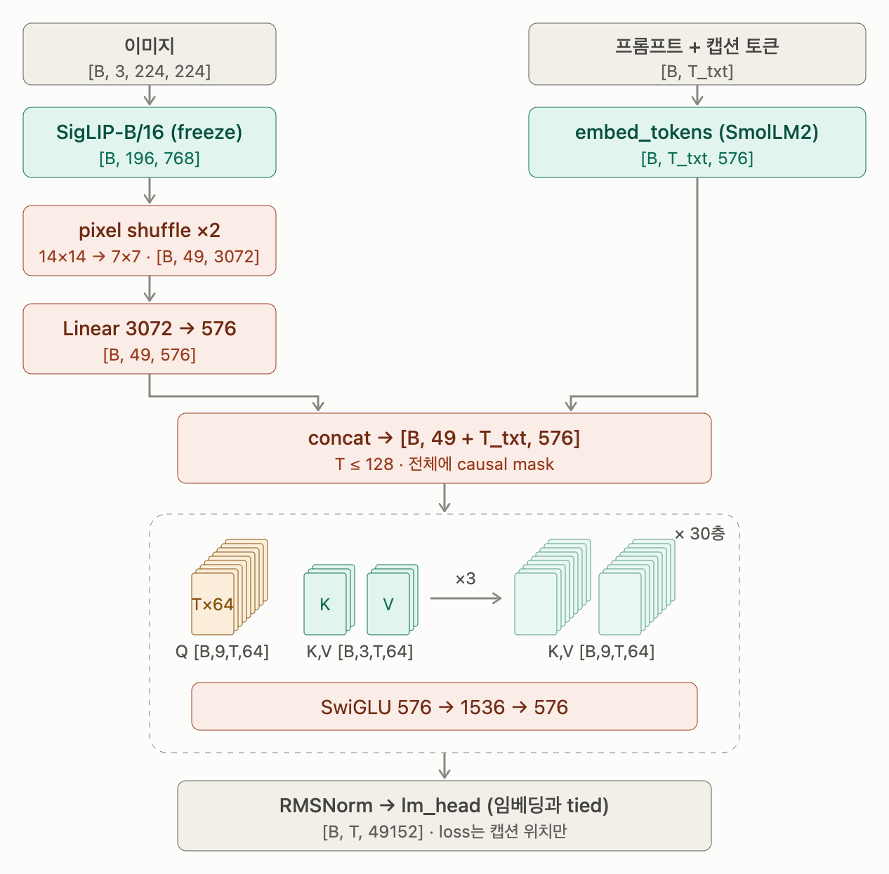
바로 들어가보자.

먼저 데이터는 허깅페이스에서 HuggingFaceM4/the_cauldron/cocoqa 를 사용하자.

HuggingFaceM4/the_cauldron · Datasets at Hugging Face

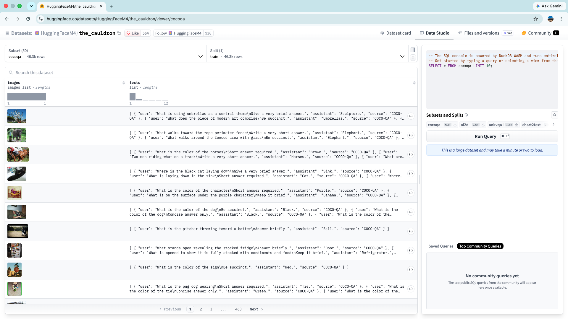
일단 항상 시작하기 전에 간단하게 데이터가 어떤 식으로 저장되어있는 지를 살펴보자.

  
from datasets import load_dataset

data = load_dataset("HuggingFaceM4/the_cauldron", "cocoqa", split="train", streaming = True)


print(data.features)
### output ####
{'images': List(Image(mode=None, decode=True)), 
'texts': List({'user': Value('string'), 
								'assistant': Value('string'), 
								'source': Value('string')})}

print("--------------------------------")

for sample in data:
    print(sample["images"][0].size)
    print(sample["texts"])
    break
    
    ### output ####
    (640, 480)
		[{'user': 'What is using umbrellas as a central theme\nGive a very brief answer.', 
			'assistant': 'Sculpture.', 'source': 'COCO-QA'}, 
			
			{'user': 'What does the piece of modern art comprise\nBe succinct.', 
			'assistant': 'Umbrellas.', 'source': 'COCO-QA'}, 
			
			{'user': 'What is this sculpture using as a central theme\nGive a very brief answer.', 
			'assistant': 'Umbrellas.', 'source': 'COCO-QA'}, 
			
			{'user': 'What is the color of the umbrellas\nQuick response, please.', 
			'assistant': 'White.', 'source': 'COCO-QA'}]

data → images, texts 가 리스트로 들어있는 상황이고, 하나의 데이터에 대해서.

image 1장 ↔ user query & answer 여러 쌍 (이미지마다 다름, 첫 샘플은 4쌍)

이 있는 상황이다.

1. Dataloading

순서는 항상 다음과 같다.

Dataset class 정의
Data loader 호출

위 데이터 스키마를 인지하고, 먼저 image의 디멘션을 확인하자. 우리가 쓸 인코더의 input은 [B, 3, 224, 224]이다. (이후에 processor가 알아서 우리가 원하는 인코더 인풋 디멘션으로 바꿔준다~ eZY)

  
#우리의 사용 모델 계획.
encoder    google/siglip-base-patch16-224 # [B, 3, 224, 224]
decoder    HuggingFaceTB/SmolLM2-135M-Instruct
tokenizer  HuggingFaceTB/SmolLM2-135M-Instruct

자 그렇다면 맨처음에 우리가 할꺼는 바로, Dataset class정의 → data loader 정의이다. 그전에 이제 토크나이저랑 processor를 호출하자.

  
def train_main():
    
    from transformers import AutoTokenizer, SiglipImageProcessor
    tokenizer = AutoTokenizer.from_pretrained("HuggingFaceTB/SmolLM2-135M-Instruct")
    processor = SiglipImageProcessor.from_pretrained("google/siglip-base-patch16-224")

    ...

여기서 이제 Dataset → split을 보면 이상적으로는 train / val / test 이렇게 3가지로 분리가 되어야하는데, 그렇지 않은 상황;; 당황하지 않고, train 하나만 가지고 train / val 로 나누어서 진행하자.

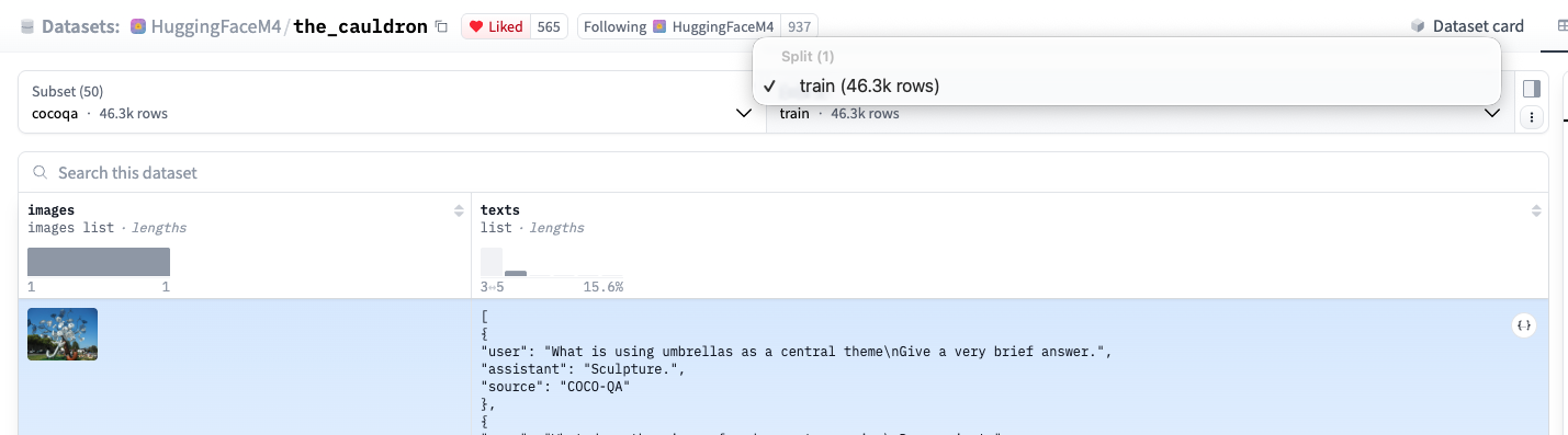
여기서, 9 : 1 의 비율로 이제 train / val 비율로 나누어주자. 이제 Dataset class를 정의에 들어가자.

자세히 보면 총 4개의 input 을 넣어주었다. (설계하는 사람이 원하는 대로 정의하면 된다) data, indices, tokenizer, processor 각각 어떻게 쓰이는지 이제부터 class를 정의하면서 살펴보자.

  
data = load_dataset("HuggingFaceM4/the_cauldron", "cocoqa", split="train")
N = len(data)

train_data_indices = range(0, int(N * 0.9))
val_data_indices = range(int(N * 0.9), N)

train_ds = VLMDataset(data, train_data_indices, tokenizer, processor)
val_ds = VLMDataset(data, val_data_indices, tokenizer, processor)

class를 정의할때 핵심은 결국에 우리가 이후에 모델 학습을 진행할때, index 즉 데이터의 번호만 주면 원하는 model input들이 나와야한다. 또한 학습을 위해서는 label(정답지)도 데이터로부터 바로 추출되어야한다.

  
class VLMDataset(torch.utils.data.Dataset):
    def __init__(self, data, data_indices, tokenizer, processor):
        self.data = data
        self.tokenizer = tokenizer
        self.processor = processor
        self.data_indices = data_indices

        # 이 부분이 굉장히 재미있는 부분이고, 결국에 data 1개 -> 여러개의 pair로 추출
        texts = data.select_columns(["texts"])["texts"]
        self.pairs = []
        for indic in data_indices:
            for turn_i in range(len(texts[indic])):
                self.pairs.append((indic, turn_i))

    def __len__(self):
        return len(self.pairs)

    def __getitem__(self, idx):
        '''
        output schema !!! token not embeddings !!
        {   
            "pixel_values": [3,224,224], (just bf the encoder)
            "input_ids": [user_tokens | assistant_tokens] (L)
            "labels"   : [-100's | answer_tokens] (L)
        }
        '''

중요한점은 데이터 1개를 → 여러개의 pair로 추출하는 작업을 반복문으로 진행해주는 것, 그리고 이제 get item에서 우리가 원하는 output schema를 확인해보자.

  
#one of the text in the data.
{'user': 'What is using umbrellas as a central theme\nGive a very brief answer.', 
			'assistant': 'Sculpture.', 'source': 'COCO-QA'}, 

우리가 여기서 {user | assistant } 를 이제 우리는 학습용 input으로 넣을 것이고, 이제 {assistant}를 정답 라벨로 사용한다는 것을 인지해야한다. 그렇기에 labels에서 우리는 -100으로 user token부분을 채워넣어주는 것. 이후에 loss를 계산할때 그게 어떻게 쓰이는지를 살펴보자.

아래 getitem은 복잡해 보이지만, 사실 아주 간단하게 우리가 원하는 schema로 바꿔주는 함수이다.

  
def __getitem__(self, idx):

    indic, turn_i = self.pairs[idx]
    raw = self.data[indic]

    turn = raw["texts"][turn_i]
    image = raw["images"][0]

    #Image -> pixel values by processor
    pixel_values = self.processor(image, return_tensors="pt")["pixel_values"][0]

    # Tokenizer makes user + assistant -> input_ids.
    input_ids = self.tokenizer.apply_chat_template(
        [
            {"role": "user", "content": turn["user"]},
            {"role": "assistant", "content": turn["assistant"]},
        ],
        tokenize=True, add_generation_prompt=False, return_tensors="pt",
    )["input_ids"][0]                                                       # [L]

    # we need user prompt length.
    prompt_len = self.tokenizer.apply_chat_template(
        [{"role": "user", "content": turn["user"]}],
        tokenize=True, add_generation_prompt=True, return_tensors="pt",
    )["input_ids"].size(1)

    # user prompt -> -100 for the loss calculation.
    labels = input_ids.clone()
    labels[:prompt_len] = -100

    output = {
        "pixel_values": pixel_values,
        "input_ids": input_ids,
        "labels": labels,
    }

    return output

자 여기서 이제 데이터 로더를 통해서, 데이터들을 이제 호출하는 것이 핵심이다. 그런데 이제 collate_fn 이라는 input 을 잘 봐보면 collate_fn=make_collate(tokenizer.pad_token_id) 하나의 함수와 pad token id가 같이 들어간 것을 알 수 있다.

  
from torch.utils.data import DataLoader

train_ds = VLMDataset(data, train_data_indices, tokenizer, processor)
val_ds = VLMDataset(data, val_data_indices, tokenizer, processor)

train_loader = DataLoader(train_ds, batch_size=16, shuffle=True, num_workers=8, collate_fn=make_collate(tokenizer.pad_token_id), drop_last=True)
val_loader = DataLoader(val_ds, batch_size=16, shuffle=True, collate_fn=make_collate(tokenizer.pad_token_id),
                        generator=torch.Generator().manual_seed(0))

이 부분이 이제 데이터 처리에서 마지막 후처리인데, 패딩을 넣어주는 부분이다. 패딩은 우리가 데이터들마다 토큰 길이가 다르지만, 하나의 배치에 대해서는 동일한 길이로 맞춰주기 위해서 (그래야 Batch 연산이 가능해진다.) 일부러 짧은 글들에 뒤에다가 토큰을 붙여주는 것이다.

여기서 패딩을 이제 채우는 역할을 이제 collate 함수에서 진행한다. 핵심은 각 배치들마다 최대길이 토큰이 다르기 때문에 그 길이를 추출하고, 그보다 짧은 토큰들을 패딩으로 채워주는것 !!!

중요한 점은 padding을 이제 input ids 즉 입력 토큰의 경우 2라는 숫자로 넣어주고, 그리고 이제 labels는 똑같이 -100으로 넣어서 아예 loss function이 계산이 안되도록 만들어준다.

	pad 값	이유
`input_ids`	`2` (pad_token_id)	모델 입력이라서 embedding 표에서 조회 가능한 실제 토큰 번호.
`labels`	`-100`	cross-entropy는 `-100`인 칸을 건너뜀.

2. Collate - data processing

정의한 make_collate 함수 내부에 collate라는 함수를 만들어주고, 이 함수는 말 그대로 기존 batch → trainable batch로 바꿔주는 역할을 한다.

  
def make_collate(pad_token_id):
    def collate(batch):
        '''
        batch -> new batch for the training the model.
        that's the purpose of the collate function.
        '''
        
        #batch 내부에서 최대 길이 토큰을 얻는다.
        max_token_len = max(data["input_ids"].size(0) for data in batch)
        attention_masks = []
        for data in batch:
            input_ids = data["input_ids"]
            labels = data["labels"]

            # 전체 길이가 max_token_len = padding token id 로 먼저 채워넣는다.
            # label(정답지)는 패딩 자리 또한 -100으로 채워넣는다.
            new_ids = torch.full((max_token_len,), pad_token_id, dtype=input_ids.dtype)
            new_labels = torch.full((max_token_len,), -100, dtype=labels.dtype)
            new_ids[:input_ids.size(0)] = input_ids
            new_labels[:labels.size(0)] = labels

            # 이제 기존의 데이터를 집어 넣어주면 완성.
            data["input_ids"] = new_ids
            data["labels"] = new_labels

            # 마지막으로 패딩 자리를 마스크로 제작해야한다.
            # 진짜 토큰 = 1, pad = 0 (pad 를 모델이 안 보게)
            # 이렇게 해야 이제 attention 연산할때 padding을 지나친다.
            new_mask = torch.zeros(max_token_len, dtype=torch.long)
            new_mask[:input_ids.size(0)] = 1
            attention_masks.append(new_mask)

        # dict 리스트 -> 텐서 dict (B 개를 쌓아서 [B, ...])
        return {
            "pixel_values": torch.stack([data["pixel_values"] for data in batch]),   # [B, 3, 224, 224]
            "input_ids": torch.stack([data["input_ids"] for data in batch]),         # [B, L]
            "labels": torch.stack([data["labels"] for data in batch]),               # [B, L]
            "attention_mask": torch.stack(attention_masks),                          # [B, L]
        }

    return collate

이후에 이제 할일은 val_batch는 고정을 해주는 일이다. 그냥 20개의 배치를 아예 고정해준다. 그래야 시험지가 똑같이 매번 채점을 하기 때문.

  
from itertools import islice
val_batches = list(islice(val_loader, 20))

3. Model call, optimizer, and scheduler

이제 모델을 호출하고, optimizer, scheduler을 호출한다.

(스케줄러란 learning rate를 training step 마다 정해진 규칙대로 조절해주는 역할을 진행한다)

  
#Model
from transformers import AutoModelForCausalLM
model = VLM(cfg).to(cfg.device)
params = [p for p in model.parameters() if p.requires_grad]
print(f"trainable params: {sum(p.numel() for p in params):,}", flush=True)
#optimizer
from torch.optim import AdamW
optimizer = AdamW(params, lr=cfg.lr)
from transformers import get_cosine_schedule_with_warmup
scheduler = get_cosine_schedule_with_warmup(optimizer, cfg.warmup_steps, cfg.training_steps)

(일단 모델에 관한 이야기는 마지막에 학습루프를 설명하고 뒤에 하도록 하겠다~)

여기서 training loop 에 들어가기전에 두가지 함수를 정의해주자.

먼저 to device 라는 함수는 batch연산을 진행하기전에 device = cpu or gpu 로 옮기는 함수이다. 연산전에 필수이므로 미리 제작해두자.

  
def to_device(b):
    return {k: v.to(cfg.device) for k, v in b.items()}

이제 training 중간중간에 미리 만들어놓은 채점표를 기준으로 loss가 얼마인지를 계산해주자.

(이걸로 학습이 잘 진행 되고 있는지 아닌지를 체크하자.)

  
def val_loss():
     model.eval()
     total = 0.0
     with torch.no_grad():
         for b in val_batches:
             total += model(**to_device(b)).loss.item()
     model.train()
     return total / len(val_batches)

4. Train loop

이제 학습 루프로 들어가서, 나온 결과들을 ./result 파일에 저장해주고, history에 train loss, val loss를 구분해서 저장해주자.

  
# Training loop
from pathlib import Path
OUT = Path(__file__).parent / "result"
OUT.mkdir(exist_ok=True)
best = float("inf")
hist = {"train_loss": [], "val_loss": []}

import time, json
t0 = time.time()
it = iter(train_loader)

for step in range(1, cfg.training_steps + 1):

    try:
        batch = next(it)
    except StopIteration:
        it = iter(train_loader)
        batch = next(it)

    loss = model(**to_device(batch)).loss

    optimizer.zero_grad()
    loss.backward()
    torch.nn.utils.clip_grad_norm_(params, 1.0)
    optimizer.step()
    scheduler.step()

자세히 보면 try: batch = next(it) except 이 부분이 재미있는게, 데이터를 우리는 it instance가 섞은 다음에 여러배치들로 만들었고 거기서 next 메서드를 호출하면 학습하지 않은 배치가 하나 튀어 나온다. 여기서 만약에 모든 배치가 다 학습이 되었다면, 여기서 에러를 발생시키고 이때는 it가 다시한번 모든 데이터에 대해서 섞고 새롭게 배치를 짜야한다. (1 epoch)를 돈것과 마찬가지다.

이 부분도 재미있는게, 이제 gradient가 1.0보다 넘지 않도록 설정해주는 부분이다. 정확히는 모든 파라미터의 gradient를 합친 전체 크기(norm)가 1.0을 넘으면, 방향은 그대로 두고 길이만 1.0으로 줄여준다.

  
torch.nn.utils.clip_grad_norm_(params, 1.0)

5. Result

단계	학습 대상	목적
Stage 1	connector만	이미지 → LLM 언어로 정렬
Stage 2	connector + LLM (전체 또는 LoRA)	이미지를 보고 대화하고 추론하는 능력

(총 2가지 학습을 진행하였다. Stage 1 → Stage 2 순서로, Stage 2는 Stage 1 에서 이어서 학습.)

5-1. Stage 1 결과 (connector 만 학습)

학습 환경과 설정은 아래와 같다.

항목	값
GPU	RunPod A40 (48GB) 1장, Secure cloud ($0.59/hr)
학습 시간	약 16.5분 (3000 step ÷ 3.04 it/s), 데이터 다운로드 + eval 포함 pod 전체 약 31분 (약 $0.30)
Steps / batch	3000 step, batch 16 (= 48,000 샘플)
Optimizer	AdamW, lr 1e-3, warmup 100 step + cosine, grad clip 1.0
학습 파라미터	442,944개 (connector `Linear(768, 576)` 하나) / 전체 227,842,176개 → 약 0.2% 만 학습
데이터	cocoqa 46,287장 → 이미지 기준 9:1 split (train 41,658장 / val 4,629장)

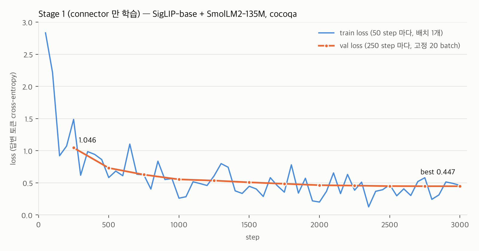
step	250	500	1000	2000	3000
val loss	1.046	0.732	0.554	0.464	0.447 (best)

connector 하나만 학습했는데도 val loss가 1.05 → 0.45 까지 내려갔다.
overfit 없이 끝까지 내려갔고, 2500 step 이후로는 거의 평평하다 (0.450 → 0.447). connector 하나로 낼 수 있는 한계에 가까워진 것.
마지막 train loss 0.46 ≈ val 0.45 → train / val 차이가 거의 없다.

5-2. Stage 2 결과 (connector + LLM 학습)

Stage 1 에서 달라진 건 딱 4가지다.

LLM requires_grad = True (SigLIP 은 계속 얼림)
Stage 1 에서 학습한 connector (best.pt) 를 불러와서 이어서 시작
lr 두 그룹: connector 1e-4, LLM 2e-5 (LLM 은 이미 잘 학습돼 있어서 아주 작게)
저장: connector + LLM 같이 → stage2_best.pt (약 540MB)

항목	값
GPU	RunPod A40 (48GB) 1장, Secure cloud ($0.59/hr)
학습 시간	약 20.7분 (3000 step ÷ 2.41 it/s), pod 전체 약 30분 (약 $0.30)
Steps / batch	3000 step, batch 16 (Stage 1 과 동일)
학습 파라미터	134,957,952개 (connector + LLM 전체) ← Stage 1 의 약 300배

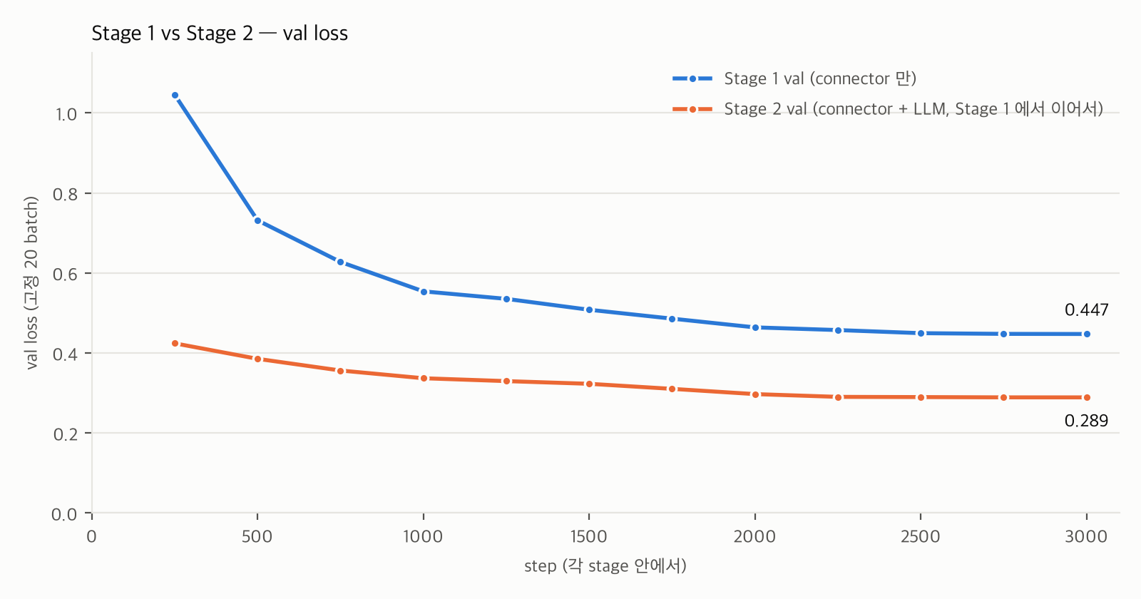
	시작 val	최종 val (best)	마지막 train loss
Stage 1 (connector 만)	1.046	0.447	0.46
Stage 2 (connector + LLM)	0.424	0.289	0.10

Stage 2 는 첫 val 이 0.424 로 Stage 1 마지막 값(0.447) 근처에서 시작했다 → connector 가 제대로 불러와졌다는 증거.
val 이 0.447 → 0.289 까지 더 내려갔다. connector 하나로는 막혔던 한계를 LLM 을 풀어서 뚫은 것.
대신 train 0.10 vs val 0.29 로 차이가 생겼다. LLM 을 풀면서 외우는 능력도 커진 것 (아직 val 이 다시 올라가지는 않아서 overfit 까지는 아님).

6. Eval (token generation)

  
@torch.no_grad()
def generate(self, pixel_values, gen_ids, eos_id, max_new_tokens=20):
    '''pixel_values [1, 3, 224, 224], gen_ids [1, L_prompt] (assistant\\n 까지) -> 답변 token id list'''
    
    # Embedding들을 이어 붙여서 하나로 만든다.
    inputs_embeds = torch.cat([self.image_embeds(pixel_values), self.lm.get_input_embeddings()(gen_ids)], dim=1)
    
    # prefill 인풋 임베딩임!!!!
    out = self.lm(inputs_embeds=inputs_embeds, use_cache=True)          
    cache, answer = out.past_key_values, []
    
    # decode (새 토큰 1 개 + cache)
    for _ in range(max_new_tokens):                                     
        next_id = out.logits[:, -1, :].argmax(dim=-1, keepdim=True)
        if next_id.item() == eos_id:
            break
        answer.append(next_id.item())
        
        # 인풋 토큰임!!
        out = self.lm(input_ids=next_id, past_key_values=cache, use_cache=True)
        cache = out.past_key_values
    return answer

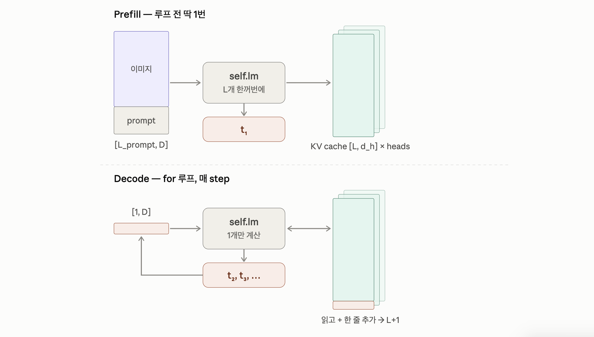
여기서 처음 보면 이상한 점이 하나 있다. 왜 self.lm을 for문 밖에서 한 번 먼저 호출하고, 그다음에 for문으로 들어갈까? 바로 for문으로 들어가면 안 되나?

답은 루프 본문의 순서에 있다. 루프 안을 보면 out에서 다음 토큰을 먼저 꺼내고 (out.logits[:, -1]), 그다음 self.lm을 호출한다. 즉 루프는 “이미 있는 out을 소비하고 → 다음 out을 만든다”는 구조다. 그래서 첫 바퀴에 들어가는 순간 이미 out과 cache가 있어야 한다. 이걸 만들어 주는 게 루프 앞의 한 번, prefill이다.

수치해석 비유: time stepping 루프 u_{n+1} = f(u_n) 에 들어가기 전에 초기조건 u_0를 먼저 세팅하는 것과 똑같다. prefill = u_0 세팅, decode = time step 반복.

6-1. Stage 1 eval 결과 (정답률 60.7%)

학습 때 한번도 안 본 val 이미지 300장 (이미지마다 첫 번째 질문)으로 답변을 생성하고, 정답이랑 그대로 비교했다 (exact match).

정답률 60.7% (182 / 300)

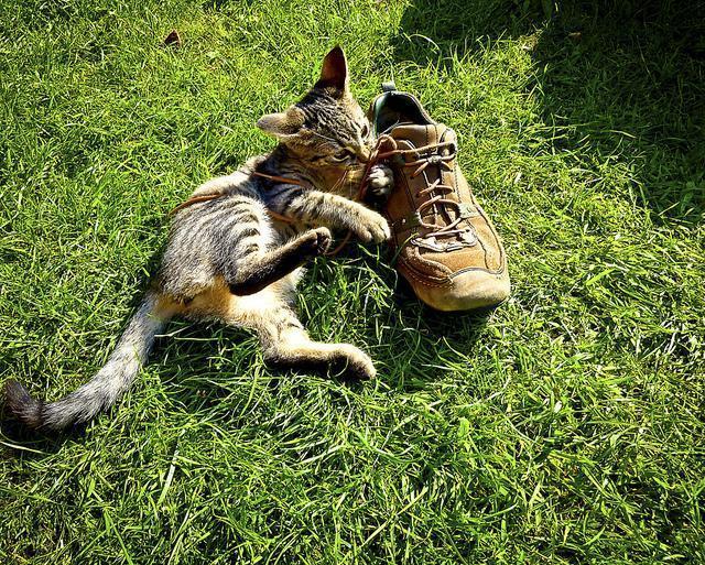
실제로 넣었던 이미지랑 prompt → 결과를 맞은 것 / 틀린 것 하나씩 보자.

✅ 맞은 예시

[user]      What is laying in the grass next to a shoe
            Give a very brief answer.
[assistant] Cat.        ← 모델 생성
[정답]      Cat.

신발 옆에 누워있는 고양이를 정확히 맞춘다.

❌ 틀린 예시

[user]      What is the color of the grass
            Write a very short answer.
[assistant] Green.      ← 모델 생성
[정답]      Brown.

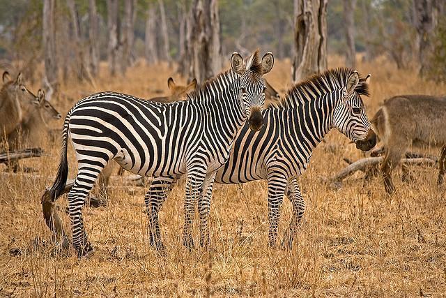
사진을 보면 풀이 메말라서 갈색인데, 모델은 Green 이라고 답했다. 이미지를 보기보다는 “풀 = 초록” 이라는 LLM의 상식을 따라간 것.

나머지 예시들을 표로 정리하면 아래와 같다.

	질문	예측	정답
O	What is laying in the grass next to a shoe	Cat.	Cat.
O	What is parked next to the truck	Motorcycle.	Motorcycle.
O	How many men stand in front of a private plane	Two.	Two.
O	What are walking around the small zoo enclosure	Giraffes.	Giraffes.
X	What is the color of the grass	Green.	Brown.
X	How many birds standing near the edge of a body of water	One.	Two.
X	What walks through the snow	Cars.	Skis.

틀린 패턴을 보면

상식으로 찍기: “풀 색깔?” → Green. 실제 사진은 갈색 풀인데 이미지보다 LLM이 원래 알던 상식을 따라갔다.
개수 세기: One / Two 를 헷갈린다. 196개 패치를 Linear 하나로만 옮겨서 세밀한 정보가 덜 넘어간 것으로 보인다.
답 형식은 완벽: 전부 “단어.” 형태로 짧게 답하고 <|im_end|> 에서 멈춘다. LLM이 이미 채팅 형식을 알고 있기 때문.

이 결과 (val 0.447 / 정답률 60.7%)가 이후 Stage 2 (LLM 까지 학습) 랑 비교할 기준선이다.

6-2. Stage 2 eval 결과 (정답률 71.3%)

Stage 1 과 똑같은 val 이미지 300장, 똑같은 질문으로 비교했다.

정답률 71.3% (214 / 300) ← Stage 1 60.7% 에서 +10.6%p

질문	정답	Stage 1	Stage 2
How many birds standing near the edge of a body of water	Two.	One. ❌	Two. ✅
Where are some black animals eating pumpkins	Pen.	Tower. ❌	Pen. ✅
What is laying in the grass next to a shoe	Cat.	Cat. ✅	Kitten. ❌ (의미는 맞음)
What is the color of the grass	Brown.	Green. ❌	Green. ❌
What walks through the snow	Skis.	Cars. ❌	Car. ❌

보면

개수 세기가 좋아졌다: Stage 1 에서 틀렸던 새 두 마리(Two)를 맞췄다. LLM 이 이미지 토큰을 더 잘 읽게 된 것.
Kitten vs Cat: 사진은 실제로 아기 고양이라 의미는 맞는데 exact match 라서 틀린 걸로 채점됐다. 채점 방식의 한계도 같이 보인다.
풀 색깔 (Green) 은 여전히 틀린다: “풀 = 초록” 이라는 상식이 아직 이미지보다 강하다.

7. Model architecture

정의한 모델 아키텍쳐에 대해서 이야기를 해보자. 이전 시간과 다르게 직접 Transformer inner 구조를 다루지는 않고, 호출하는 방식을 선택하였다. 일단 호출한 모델은 ‘encoder’ and ‘decoder’ 이다.

  
class VLM(torch.nn.Module):
    '''
    main() 에서 한 흐름을 클래스로 묶은 것.
    [img x196 | text] -> SmolLM2 -> logits / loss
    '''
    def __init__(self, cfg: Config):
        super().__init__()
        from transformers import SiglipVisionModel, AutoModelForCausalLM
        self.vision = SiglipVisionModel.from_pretrained("google/siglip-base-patch16-224")
        self.lm = AutoModelForCausalLM.from_pretrained("HuggingFaceTB/SmolLM2-135M-Instruct", dtype=torch.float32)
        self.connector = torch.nn.Linear(768, 576)  # SigLIP hidden 768 -> SmolLM2 hidden 576 (새로 학습하는 부분)

        # Stage 1: SigLIP, LLM 얼림 (requires_grad False). no_grad 는 안 씀 -> gradient 가 LLM 을 지나 connector 까지 흐름
        for p in self.vision.parameters():
            p.requires_grad = False
        for p in self.lm.parameters():
            p.requires_grad = False # Stage1 Training
           #p.requires_grad = True # Stage2 Training

여기서 두가지 포인트가 있다.

connector : Image embedding 을 Text embedding과 결합해야하는데 이 차원을 맞춰주는 역할이다.
SigLIP encoder는 얼렸고 얼리는 방식은 requires_grad = False (굉장히 중요하다)
- Stage1 ~ 사실상 Connector 하나 학습.
- Stage2 ~ Connector + LLM (inc / lm_head)

이어서 이제 forward를 살펴보자. 우리는 토큰을 입력으로 받기 때문에

Token → Embeddings

이게 핵심 목표이다.

  
  def __init__(self, cfg: Config):
      ...

# image tensor -> (encoder) -> image embeddings -> (connector) -> new image embeddings
  def image_embeds(self, pixel_values: torch.Tensor) -> torch.Tensor:
      with torch.no_grad():                                               # vision 앞에는 학습할 게 없어서 no_grad OK
          h = self.vision(pixel_values=pixel_values).last_hidden_state    # [B, 196, 768]
      return self.connector(h)                                            # [B, 196, 576]

  def forward(self, pixel_values, input_ids, attention_mask, labels=None):
      img = self.image_embeds(pixel_values)                               # [B, 196, 576]
      txt = self.lm.get_input_embeddings()(input_ids)                     # [B, L, 576]
      B, N = img.shape[:2]

      inputs_embeds = torch.cat([img, txt], dim=1)                        # [B, 196 + L, 576]
      attention_mask = torch.cat([attention_mask.new_ones(B, N), attention_mask], dim=1)   # 이미지는 항상 1
      if labels is not None:
          labels = torch.cat([labels.new_full((B, N), -100), labels], dim=1)               # 이미지는 채점 X
      return self.lm(inputs_embeds=inputs_embeds, attention_mask=attention_mask, labels=labels)

여기서 중요한점은 image 임베딩만 connector을 거쳐서 text 와 동일한 디멘션(576)의 임베딩으로 바꿔준다는 것이다. text는 LLM 안에 있는 embedding 표를 그대로 쓴다.

그리고 이제 text embedding과 concat 합쳐준다. (dim=1 시퀀스 축으로 앞뒤로 이어 붙인다 → [img 196개 | text L개])

이제 one of the most important attention_mask의 경우에는 이제 전체 토큰이 길어졌으니 같이 길어져야한다. 여기서 attention_mask는 causal mask가 아니라 padding mask (진짜 토큰 1, pad 0) 이고, causal mask는 HF가 내부에서 자동으로 만들어준다. 앞에 붙은 Image token은 pad가 아니라 진짜 토큰이기 때문에 그 길이(196)만큼 1을 붙여줘야한다. 그 작업을 이제 진행해주고 정답지 또한 길이를 맞춰줘야 하는데 이미지의 경우 사실 정답이 필요가 없으므로 -100으로 채워준다.

그다음에 self.lm 즉 LLM “HuggingFaceTB/SmolLM2-135M-Instruct” 에 넣어준다.

Study, AI