SmolVLA (Inference) - part2 (Action Expert)
SmolVLA 코드 분석 두번째. VLM이 만든 KV cache를 가지고 Action Expert가 노이즈에서 action chunk를 뽑아내는 denoising 루프를 따라간다. select_action과 queue, embed_suffix, causal mask, 짝수층 self-attention과 홀수층 cross-attention, 그리고 unpad와 역정규화까지 정리한다.
실습 목표 자체는 실제로 VLA의 코드를 뜯어 분석해보는 것이다. (lerobot → SmolVLA)
- Inference
- VLM (이전시간)
- Action Expert (이번시간)
- Training (다음시간)
SmolVLA: A vision-language-action model for affordable and efficient robotics
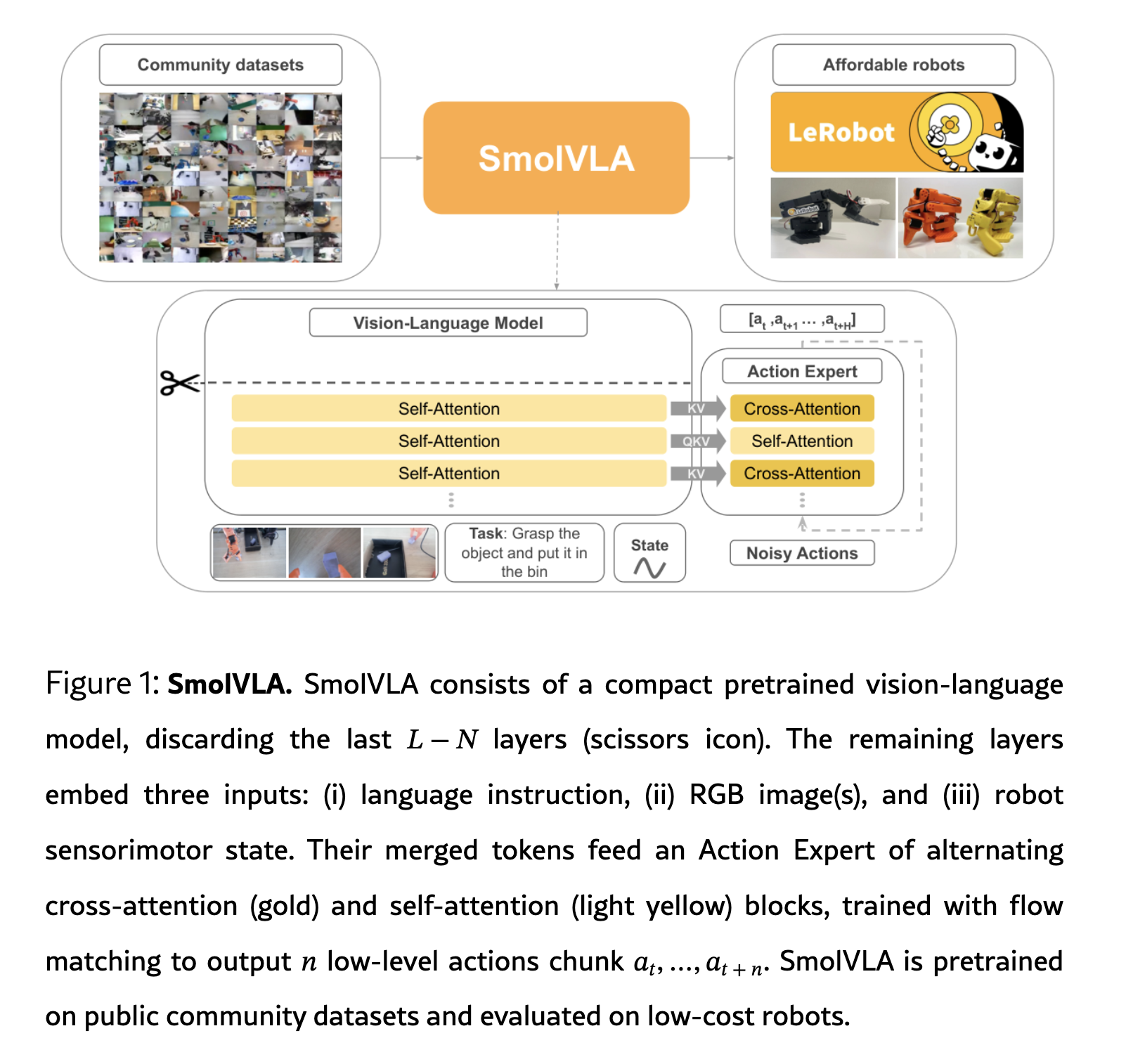
VLA중에서 가장 흠… 저렴한 그리고 가벼운 VLA → SmolVLA를 운이 좋게 발견하였다. lerobot이라는 커뮤니티라고 해야할까? 곳에서 로봇의 학습을 중요시하고 저렴한 모델과 로봇, 그리고 데이터셋을 공개해주는 아주 착한 커뮤니티이다.
지난시간에는 우리가 추론단계에서도 VLM 즉 앞 쪽 부분을 코드를 뜯어보면서 분석했었다.
오늘 today , jintian은 SmolVLA lerobot 코드 분석 두번째 시간에는 이제 오른쪽 Action 루프에 대해서 탐구를 진행해보자.
Overall workflow
(지난시간 리마인더)
결국 우리가 받는 image, prompt , state → 를 가지고 원하는 관절값 액션을 뽑아내야한다. 여기서 대부분까지는 아니어도 다들 “아 우리가 pre-trained된 VLM을 가져다 쓰자”라고 이 VLA연구들이 시작되었다. 따라서, 사전학습된 VLM에 넣고, 그리고 얻어낸 16개 self attention layer마다의 Key, Value vector을 Cache에 저장해서 그대로 Action Expert의 self attention layer and cross attention layer에다가 넣어준다.
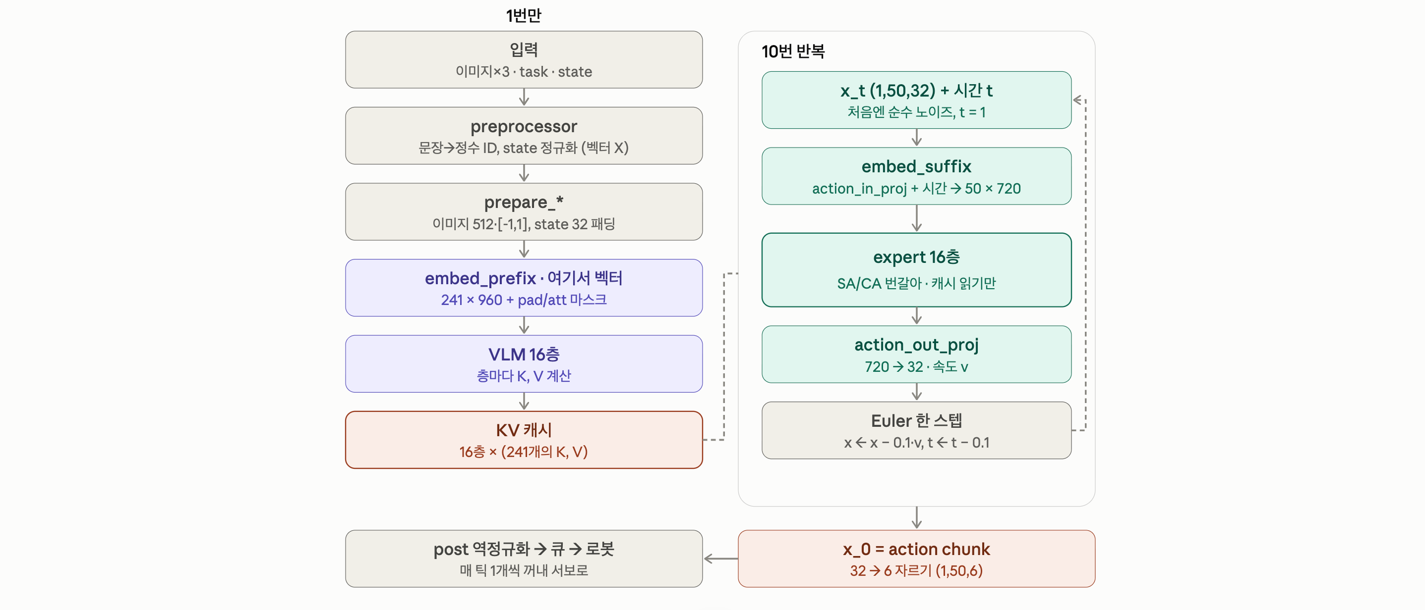
핵심은 Action expert loop을 Denoising 이라고 칭한다. Diffusion model과 비슷하게 노이즈 → 우리가 원하는 액션으로 바꾸는 그렇게 학습된 모델이기 때문이다.
여기서 Query = {action_token} 이고 이제 Key, Value는 {Image, Language, state, Action}을 전부 포함하거나, Action은 제외되거나에 따라서 self attention, cross attention이 갈리는 것이다.
(사실 이렇게 말할 수 있는 것도 한바퀴를 분석을 진행하고 돌아왔기 때문이다… 맨처음에 저 루프를 볼때, 아니 뭐가 뭔지 잘 몰랐다… 일단 질문을 가지고 밑에 분석에 들어가보자)
정확히 우리가 로봇의 관절값을 뽑을때, Image, task, state를 참고를 할 것인데 어떻게 참고를 하도록 설계가 되어있는가??
아 들어가기전에 나도 배우면서 알게된 용어정리를 한번하고가자.
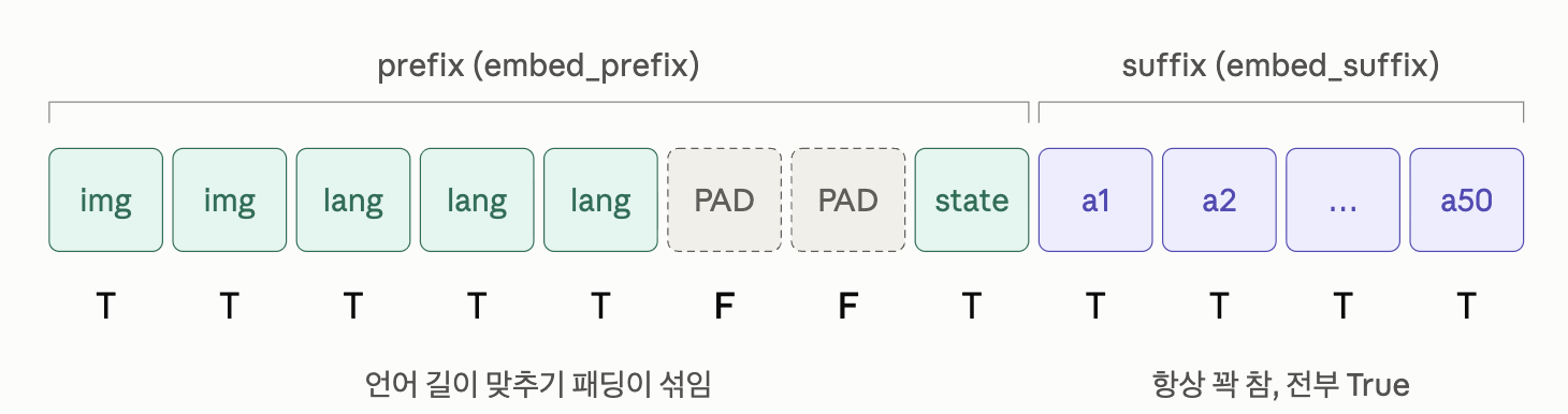
- prefix : { Image, Language, State } tokens → 192 + 48 + 1 = 241 tokens (960-dim)
- suffix : { Action } tokens → 50 tokens (720-dim, noisy action + time)
prefix 가 접두사, suffix가 접미사라는 것도 처음알았다. 이게 VLM에서 input으로 들어가는게 prefix 그 뒤에 denoising action expert model에 input으로 들어가는 것을 suffix라고 칭하는 것이다.
(코드 주석에는 저 용어로 정리되어있고, 이 분야에서는 consensus하게 저 용어를 쓰는 것을 확인하였다)
자 이제 들어가기전에, Flow Matching 개념 진짜 한번만 보고 가자
0. (Review) Flow matching
Action Expert가 하는 일은 한 줄로 요약하면,
“노이즈에서 액션으로 가는 속도장(velocity field)을 예측하는 것”
Diffusion과 같은 생성 모델 계열이지만, 노이즈와 데이터 사이를 직선 경로로 잇고 그 경로 위의 속도를 배운다는 점이 다르다.
“지난시간 Flow matching 블로그에서 굉장히 강조한 부분은 바로,
학습: 직선 경로 위의 속도를 배운다 는 것”
SmolVLA(lerobot) 코드 기준으로 $t=1$ 이 노이즈, $t=0$ 이 실제 액션이다. 둘을 직선으로 섞은 점 $x_t$ 를 만들고,
\[x_t = t\,\epsilon + (1-t)\,a, \qquad \epsilon \sim \mathcal{N}(0, I)\]이 직선의 속도(시간 미분)를 정답으로 둔다.
\[u_t = \frac{dx_t}{dt} = \epsilon - a\]모델 $v_\theta$ 는 관측(이미지·언어·state)을 조건으로 이 속도를 맞히도록 MSE로 학습된다. 이 $v_\theta$ 가 바로 Action Expert다.
\[\mathcal{L} = \left\| v_\theta(x_t, t \mid \text{obs}) - (\epsilon - a) \right\|^2\]추론: ODE를 Euler로 적분한다
추론 때는 정답 $a$ 를 모르니, 노이즈 $x_1$ 에서 출발해 모델이 알려주는 속도를 따라 $t=1 \rightarrow 0$ 으로 걸어간다. 결국 ODE 하나를 푸는 문제고, SmolVLA는 가장 단순한 explicit Euler를 쓴다 ($\Delta t = -0.1$, 10 step).
\[x_{t+\Delta t} = x_t + \Delta t \cdot v_\theta(x_t, t \mid \text{obs})\]이제 코드로 들어가기전에, 앞으로 다음을 기억하고 살펴보자.
- 관측(obs)은 루프 내내 변하지 않는다 → VLM은 한 번만 돌리고 KV cache로 재사용 (part1에서 만든 것)
- 루프 안에서 매번 바뀌는 건 $x_t$ 와 $t$ 뿐 → 이 둘을 토큰으로 만드는 게
embed_suffix- Expert는 “행동 자체”가 아니라 속도를 출력한다 → 출력
v_t를 Euler로 누적해야 액션이 된다- 한 번에 50 step짜리 action chunk를 통째로 생성한다
진짜로 한단계씩 살펴보자.
1. select_action → predict_action_chunk
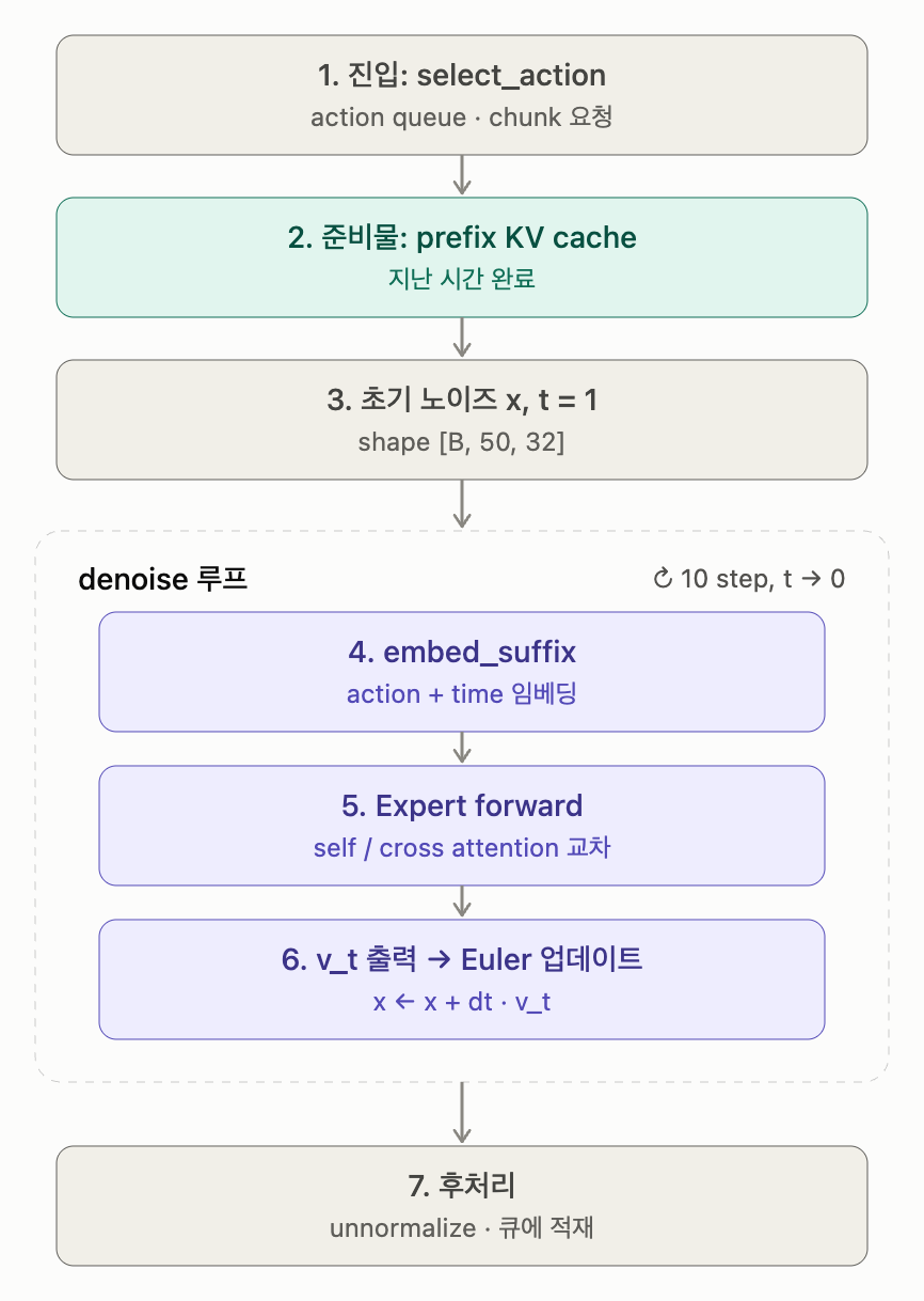
그러니까 이게 가장 중요하다, queue라는 곳은 예전에 추론해놓은 액션 리스트들이 있고, 실제로 액션이 일어난 것들은 대기목록에서 제외되는 구조이다. 여기서, 결국 추론은 큐가 비어있지 않을때는 일어나지 않는 것이 핵심적인 아이디어이다.
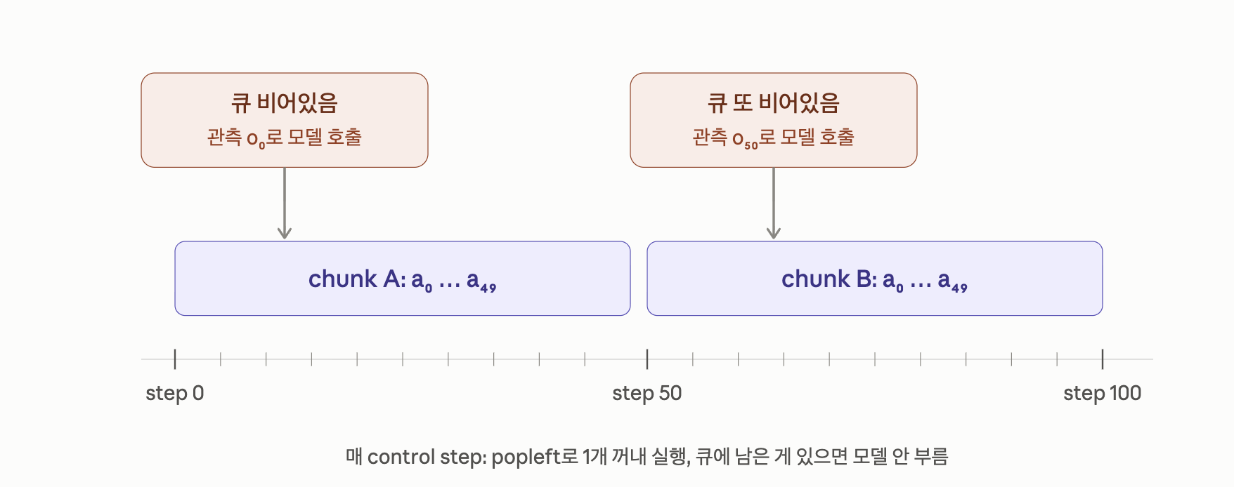
modeling_smolvla.py 를 살펴보면, SmolVLA는 queue에 액션이 다 고갈되어야 새로 호출하도록 설계가 되었다.
1
2
3
4
5
6
7
8
9
10
11
12
13
self._queues = populate_queues(self._queues, batch, exclude_keys=[ACTION])

if self._check_get_actions_condition():          # len(queue[ACTION]) == 0
    actions = self._get_action_chunk(batch, noise)  # [B, 50, A]
    self._queues[ACTION].extend(actions.transpose(0, 1)[: self.config.n_action_steps])

return self._queues[ACTION].popleft()


## 그러니까 대기중인 액션 청크가 없을때, 새로 생성.
def _check_get_actions_condition(self) -> bool:
    return len(self._queues[ACTION]) == 0
Real - Time Chunking
config 기본값이 chunk_size = 50, n_action_steps = 50이라 50개를 다 쓰고 나서야 호출이 된다. n_action_steps를 줄이면(예: 10) chunk 앞부분 10개만 실행하고 나머지 40개는 버린 뒤 새 관측으로 다시 계획한다는 것이다. 반응성은 좋아지고, 대신 모델 호출이 5배 느는 단점이 있다.
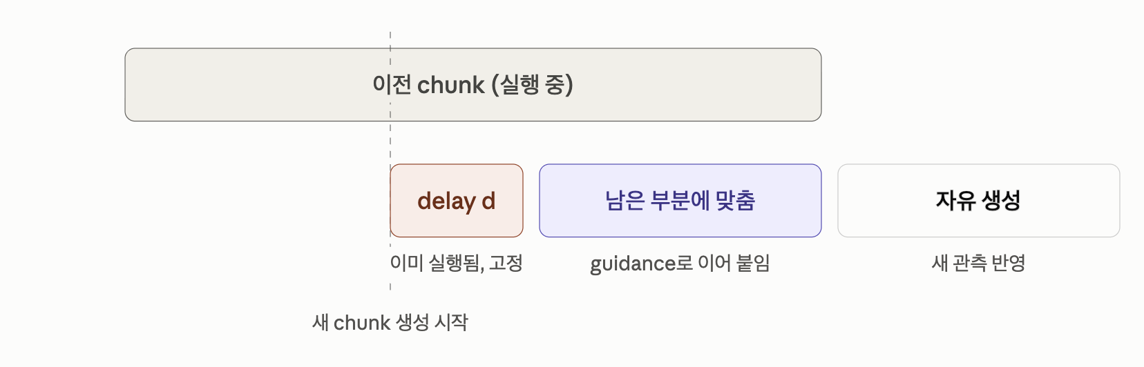
실제로 “chunk 사이를 어떻게 이어붙이냐”를 다루는 건 따로있고, 이를 우리는 RTC(Real-Time Chunking) 모드라고 부른다. 그리고 존재만 알아 놓고, 다음 블로그에서 살펴보자.
2. Prefix KV cache (part1 연결)
Action Expert가 돌기 전에 필요한 건 “관측을 이미 다 읽은 VLM의 기억”, 즉 prefix(이미지 + 언어 + state)에 대한 레이어별 Key/Value다. part1에서 본 것처럼 VLM을 한 번 forward 하면서 이걸 만들어두고, 이후 denoise 루프 10번 내내 그대로 재사용한다.
flowchart LR
    P["prefix<br>이미지 3장 + 언어 + state"] --> V["VLM forward 1회<br>16 layers, 전부 self-attn"]
    V --> C["KV cache<br>layer 0 ~ 15의 K, V"]
    C -.->|"10번 재사용"| E["Action Expert<br>denoise step"]
1
2
3
4
5
6
7
8
9
10
11
12
13
14
15
16
17
18
19
20
21
22
23
24
25
26
27
28
29
30
31
32
33
34
35
36
37
38
39
40
41
42
43
44
45
46
47
48
49
50
51
52
53
54
55
56
57
58
59
60
61
62
63
64
65
66
67
68
69
70
71
72
73
74
75
76
77
78
79
80
81
82
83
84
85
86
87
88
89
90
91
92
93
'''
Part2 -> Action Expert Attention Algorithm
'''
import torch
from lerobot.configs import PreTrainedConfig
from lerobot.policies import make_pre_post_processors
from lerobot.policies.smolvla.modeling_smolvla import SmolVLAPolicy, make_att_2d_masks
from lerobot.utils.constants import OBS_STATE, OBS_LANGUAGE_TOKENS, OBS_LANGUAGE_ATTENTION_MASK

MODEL_ID = "lerobot/smolvla_base"
DEVICE = "cpu"

# 모델 설계도(config) 다운로드: 레이어 개수, hidden size, chunk_size 등
config = PreTrainedConfig.from_pretrained(MODEL_ID)
config.device = DEVICE

# config 기반으로 policy 생성 + 가중치 로드
policy = SmolVLAPolicy.from_pretrained(MODEL_ID, config=config)
policy.eval()

# pre / post processor (정규화, 토크나이즈, device 이동)
pre, post = make_pre_post_processors(
    policy.config,
    pretrained_path=MODEL_ID,
    preprocessor_overrides={"device_processor": {"device": DEVICE}},
)

####################################
# Step1 create input
####################################
raw = {
    "observation.images.camera1": torch.rand(3, 256, 256),
    "observation.images.camera2": torch.rand(3, 256, 256),
    "observation.images.camera3": torch.rand(3, 256, 256),
    OBS_STATE: torch.rand(6),  # 6 DOF robot
    "task": "pick up the red cube and place it in the box",
}
batch = pre(raw)

####################################
# Step2 sample_actions: chunk 통째로 한 번 뽑아보기 (전체 흐름 확인용)
####################################
images, img_masks = policy.prepare_images(batch)
state = policy.prepare_state(batch)
lang_tokens = batch[OBS_LANGUAGE_TOKENS]
lang_masks = batch[OBS_LANGUAGE_ATTENTION_MASK]

with torch.no_grad():
    actions_32 = policy.model.sample_actions(images, img_masks, lang_tokens, lang_masks, state)
print("sample_actions out:", actions_32.shape)   # [1, 50, 32]

actions = actions_32[:, :, :6]                     # max_action_dim 32 → 실제 6 DOF
print("unpadded:", actions.shape)                   # [1, 50, 6]

####################################
# Step3 get past_key_values from VLM (sample_actions 앞부분을 손으로 풀어쓰기)
####################################
model = policy.model  # VLAFlowMatching

# 초기 노이즈 x_1 (다음 섹션 denoise 루프의 출발점)
bsize = state.shape[0]
noise = model.sample_noise((bsize, model.config.chunk_size, model.config.max_action_dim), state.device)
print("noise:", noise.shape)                       # [1, 50, 32]

# prefix 임베딩 + mask + position id
prefix_embs, prefix_pad_masks, prefix_att_masks = model.embed_prefix(
    images, img_masks, lang_tokens, lang_masks, state=state
)
prefix_att_2d_masks = make_att_2d_masks(prefix_pad_masks, prefix_att_masks)
prefix_position_ids = torch.cumsum(prefix_pad_masks, dim=1) - 1

# VLM만 한 번 돌려서 KV cache 채우기 (suffix 자리는 None)
with torch.no_grad():
    _, past_key_values = model.vlm_with_expert.forward(
        attention_mask=prefix_att_2d_masks,
        position_ids=prefix_position_ids,
        past_key_values=None,              # None이면 "prefill 모드" → 캐시를 새로 만듦
        inputs_embeds=[prefix_embs, None], # [VLM 입력, Expert 입력]
        use_cache=model.config.use_cache,
    )

print("layers:", len(past_key_values))     # num_vlm_layers = 16

# lerobot 버전에 따라 cache 형식이 다름
if isinstance(past_key_values, dict):      # 구버전: {layer_idx: {"key_states", "value_states"}}, [B, seq, heads, head_dim]
    k0 = past_key_values[0]["key_states"]
    v0 = past_key_values[0]["value_states"]
else:                                       # 신버전: HF DynamicCache, [B, heads, seq, head_dim]
    k0 = past_key_values.layers[0].keys
    v0 = past_key_values.layers[0].values
print("layer0 K:", k0.shape)
print("layer0 V:", v0.shape)
print("prefix len:", prefix_embs.shape[1])  # K/V의 seq 축과 같아야 함
직접 출력해서 확인해봐야 할 사항들 (직접 해보면 기억에 많이 남는다)
layers가 16: VLM 전체 레이어가 아니라 앞쪽num_vlm_layers(16)개만 쓴다- K/V의 seq 축 = prefix 길이: 이미지 토큰 + 언어 토큰 + state 토큰 1개
- heads 축은 query head 수가 아니라 KV head 수(GQA)다
- prefill 때는 cross-attn 레이어여도 전부 self-attn으로 돌아서, 16개 레이어 모두에 K/V가 채워진다
- 저장된 K는 RoPE가 이미 적용된 후의 값이다 → 나중에 expert는 이걸 다시 회전시키지 않고 그대로 읽는다
3. Denoising
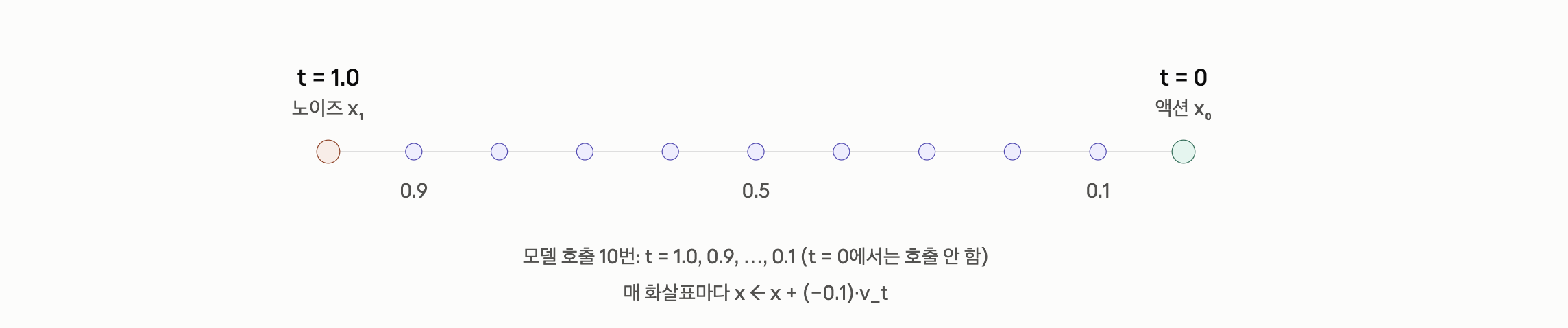
아래 반복문 코드가 사실 전부이다 ㅋㅋㅋ 굉장히 심플하다. 그냥 학습을 할때 애초에 저 현재의 prefix → KV cache, x_t (현재 위치) 그리고 time에 따라서 속도가 도출되도록 학습이 되는 것. 따라서, 이를 그냥 바탕으로 Euler one step by step 으로 점진적으로 전진을 하면 되고 그것을 10번 하면 된다.
1
2
3
4
5
6
7
8
9
10
11
12
13
14
15
16
17
18
19
20
21
22
23
24
25
26
27
28
###############################################################
########## Next step euler_integrate and denoise_step #########
###############################################################

torch.manual_seed(0)

num_steps = model.config.num_steps # 10 in here
dt = -1.0 / num_steps              # -0.1 (t changes from 1 -> 0)

x_t = noise
with torch.no_grad():
    for step in range(num_steps):
        t = 1.0 + step * dt
        time_tensor = torch.full((bsize,), t , dtype = torch.float32)

        v_t = model.denoise_step(
            prefix_pad_masks = prefix_pad_masks,
            past_key_values = past_key_values,
            x_t = x_t,
            timestep = time_tensor
        )

        x_t = x_t + dt * v_t # Euler one step

        print(f"step {step} t={t:.1f} v_t {tuple(v_t.shape)} "
              f"cache_len {past_key_values.get_seq_length()}")
자 이제 그렇다면 denoise step method, 핵심 메서드를 파헤쳐 보자.
- A: Suffix Embedding
- B: Attention Full Mask
- C: Forward
- D: Post processing
이렇게 4가지 워크플로우로 사실상 정리가 된다. 실제 코드는 다음과 같다.
1
2
3
4
5
6
7
8
9
10
11
12
13
14
15
16
17
18
19
20
21
22
23
24
25
26
27
28
29
30
31
32
33
34
35
36
37
38
39
40
41
42
43
44
45
## lerobot -> policies -> smolvla -> modeling_smolvla.py

def denoise_step(
    self,
    prefix_pad_masks,
    past_key_values,
    x_t,
    timestep,
):
    """Apply one denoising step of the noise `x_t` at a given timestep."""

    # A - Suffix Embedding suffix_embs = [B, L_s, D_s] = [1, 50, 720]
    suffix_embs, suffix_pad_masks, suffix_att_masks = self.embed_suffix(x_t, timestep)

    # B - Attention Mask
    suffix_len = suffix_pad_masks.shape[1]
    batch_size = prefix_pad_masks.shape[0]
    prefix_len = prefix_pad_masks.shape[1]
    prefix_pad_2d_masks = prefix_pad_masks[:, None, :].expand(batch_size, suffix_len, prefix_len)

    suffix_att_2d_masks = make_att_2d_masks(suffix_pad_masks, suffix_att_masks)

    full_att_2d_masks = torch.cat([prefix_pad_2d_masks, suffix_att_2d_masks], dim=2)
    prefix_offsets = torch.sum(prefix_pad_masks, dim=-1)[:, None]
    position_ids = prefix_offsets + torch.cumsum(suffix_pad_masks, dim=1) - 1

    # C - Forward (Main attention)
    outputs_embeds, _ = self.vlm_with_expert.forward(
        attention_mask=full_att_2d_masks,
        position_ids=position_ids,
        past_key_values=past_key_values,
        inputs_embeds=[None, suffix_embs],
        use_cache=self.config.use_cache,
    )

    # D - Projection
    if past_key_values is not None:
        # Self-attention layers append suffix K/V in place; restore the prefix for the next step.
        past_key_values.crop(prefix_len)
    suffix_out = outputs_embeds[1]
    suffix_out = suffix_out[:, -self.config.chunk_size :]
    suffix_out = suffix_out.to(dtype=torch.float32)
    v_t = self.action_out_proj(suffix_out)
    return v_t
하나씩 차근차근 살펴보자.
A - Suffix Embedding
Attention 연산을 하기전에 임베딩 벡터로 전환하는 것은 국룰이다.
1
suffix_embs, suffix_pad_masks, suffix_att_masks = self.embed_suffix(x_t, timestep)
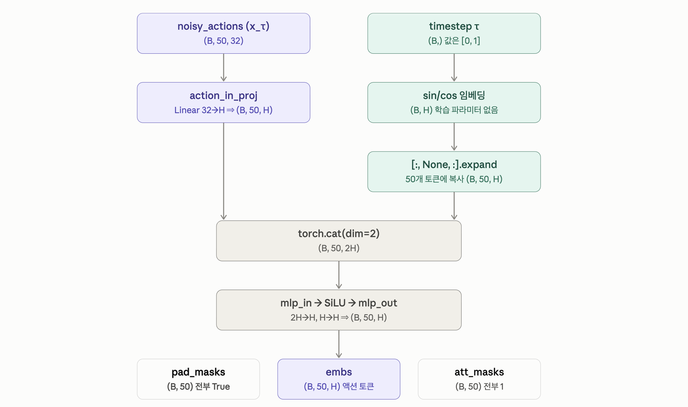
내부 코드 embed_suffix 메서드를 살펴보면, 우리는 Noisy_action , time 두가지를 다 임베딩해야하고,
time step 같은 경우 sin/cos embedding을 진행하는 것이 특징이다 + torch.cat(dim = 2) 로 두 임베딩을 합쳐준다.
최종적으로 prefix (이전) 과 동일하게 pad_masks, att_masks 그리고 embedding(720 Dimension)을 이렇게 3가지를 얻게된다. 여기서 attention masks는 전부 1인 것이 핵심이다. 지난번에 살펴봤듯이 1은 “여기서 한 층 올라간다”는 표시라서, cumsum을 하면 액션 토큰마다 한 층씩 올라간다. → 액션끼리는 자기 앞 액션까지만 보는 Causal 구조가 된다. (아래 B에서 다시 확인)
1
action_time_mask = torch.ones(bsize, action_time_dim, dtype=torch.bool, device=device)
그리고 padding을 넣지는 않았지만 우리의 prefix와 같이 나중에 작업을 하려면 그래도 만들어주고 나중에 합칠 예정이다.
그리고 (MLP: 2H → SiLU → MLP: H) 작업을 진행해서 차원을 줄여준다.
1
2
3
action_time_emb = self.action_time_mlp_in(action_time_emb)
action_time_emb = F.silu(action_time_emb)  # swish == silu
action_time_emb = self.action_time_mlp_out(action_time_emb)
1
2
3
4
5
concat           [1, 50, 1440]   (2H)
mlp_in  Linear   1440 → 720      ← 차원 축소는 여기서 (2H → H)
SiLU             720             ← 비선형성 (차원 그대로)
mlp_out Linear   720 → 720       ← H → H
                 [1, 50, 720]
결국 핵심의 아이디어는 1. 비선형성, 2. 차원축소 이 두가지가 핵심인 과정이다.
“t에 따라 액션을 다르게 해석하는” 우리는 Network를 만드는 것이 목표이기 때문.
B - Attention Mask
Prefix에서 우리가 공부를 했을때, 사실 굉장히 애매하고 어려웠던 부분중 하나이다.
결국에 핵심은 아래 질문을 위한 도구이다.
“누가 → 누구를 참고해서 Attention 연산을 진행하게 할까?”
일단 prefix pad 2d masks 는 원래 우리가 가지고 있었고, 그거를 이제 2D 로 확장시킨다.
1
prefix_pad_2d_masks = prefix_pad_masks[:, None, :].expand(batch_size, suffix_len, prefix_len)
(B, L_P) → (B, 1, L_P) → (B, 50, L_P)
그리고 지난시간에 우리가 배운 2D Mask 생성 메서드를 활용하면 suffix 2d Mask를 다음과 같이 생성할 수 있다. suffix는 Causal Mask로 생성하는 것이 여기서 특징이다.
1
2
# B - Attention Mask
suffix_att_2d_masks = make_att_2d_masks(suffix_pad_masks, suffix_att_masks)
(B, 50, P)
이제 둘이합쳐서 Full att 2d mask를 얻는다. (B, 50, 50 + P)
1
full_att_2d_masks = torch.cat([prefix_pad_2d_masks, suffix_att_2d_masks], dim=2)
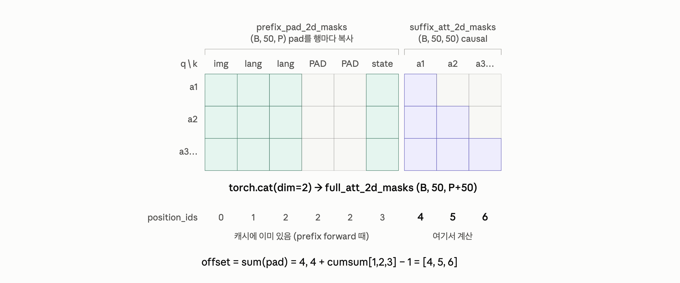
실제로 mask를 추출해보면 다음과 같다.
- 액션입장에서 image, prompt padding은 볼 필요가 없고,
- 그리고 미래 step-action은 볼 수 없기 때문에 저렇게 Causal Mask
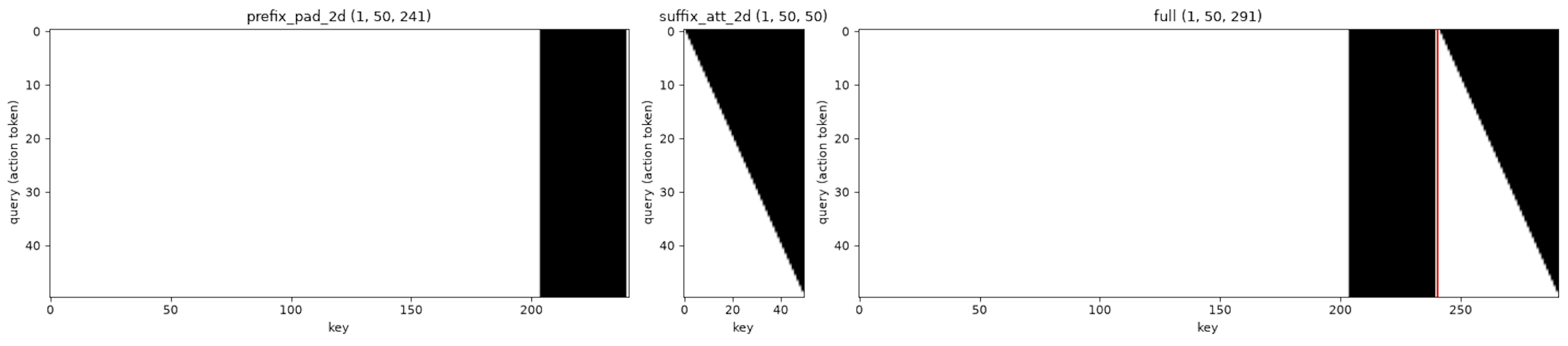
마지막으로, position_ids는 padding을 제외하고 토큰의 인덱스를 순서대로 부여해준 것 (많이 저장하면 저장공간 손해이다, 필요없는 것은 저장할 필요가 없다)
1
2
prefix_offsets = torch.sum(prefix_pad_masks, dim=-1)[:, None]
position_ids = prefix_offsets + torch.cumsum(suffix_pad_masks, dim=1) - 1
C - FORWARD
그 다음 이제 진짜 핵심 attention 연산인 Forward를 파헤쳐 보자.
1
2
3
4
5
6
7
8
# C - Forward (attention)
outputs_embeds, _ = self.vlm_with_expert.forward(
    attention_mask=full_att_2d_masks,
    position_ids=position_ids,
    past_key_values=past_key_values,
    inputs_embeds=[None, suffix_embs],
    use_cache=self.config.use_cache,
)
우리는 이제 아래의 4가지를 가지고 작업에 들어갈 예정:
- prefix + suffix → full MASK
- position ids
- KV CACHE from VLM
- input embedding(token → vector)
여기서 재미있는게 사실 우리는 KV Cache 얻는 용도로 forward를 한번 실행했었다. 여기서
inputs_embs = [prefix_embs, None]이었던 사실이 기억날 것이다. (no action chunk)
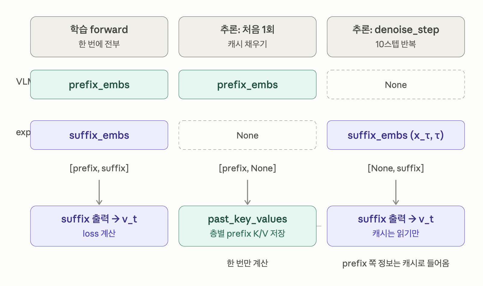
그리고 이제 그 다음 inputs_embeds 같은 경우는 오히려,
1
inputs_embeds=[None, suffix_embs]
즉 이번 Forward에서는 input_embs = suffix embs만 존재한다는 것을 인지하고 들어가보자.
1
2
3
4
5
6
7
8
9
10
11
12
13
14
15
16
17
18
19
20
21
22
23
24
25
26
27
28
29
30
31
32
33
34
35
36
37
38
39
40
41
42
43
# lerobot -> policies -> smolvla -> smolvlm_with_expert.py

def forward(
    self,
    attention_mask: torch.Tensor | None = None,
    position_ids: torch.LongTensor | None = None,
    past_key_values: "DynamicCache | None" = None,
    inputs_embeds: list[torch.Tensor | None] | None = None,
    use_cache: bool | None = None,
):

    # Two models we have.
    models = [self.get_vlm_model().text_model, self.lm_expert]
    model_layers = self.get_model_layers(models)

    # 이번에는 이거 False임 past_key_values not None 이니까
    fill_kv_cache = use_cache and past_key_values is None
    if fill_kv_cache:
        past_key_values = DynamicCache()

    # RMSNorm
    num_layers = self.num_vlm_layers
    head_dim = self.vlm.config.text_config.head_dim

    # 여기서 재밌는게, 짝수층이면 -> layer_idx % self.self_attn_every_n_layers == 0
    for layer_idx in range(num_layers):

        # 짝수층
        if (
            fill_kv_cache  # 이번에는 False
            or "cross" not in self.attention_mode
            or (self.self_attn_every_n_layers > 0 and layer_idx % self.self_attn_every_n_layers == 0)
        ):
            att_outputs, past_key_values = self.forward_attn_layer(
                ...
            )

        # 홀수층
        else:
            att_outputs, past_key_values = self.forward_cross_attn_layer(
                ...
            )
여기서 이제 우리가 짝수층 홀수층 다르게 self attention, cross attention을 진행하는게 SmolVLA의 가장 큰 특징이었다.
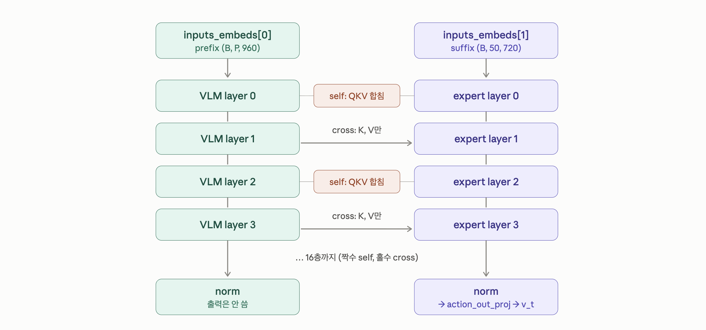
자 지난시간에는 forward_attn_layer method만 살펴보았는데, 이번에는 둘다 쓰이므로 둘다 파헤쳐 보자.
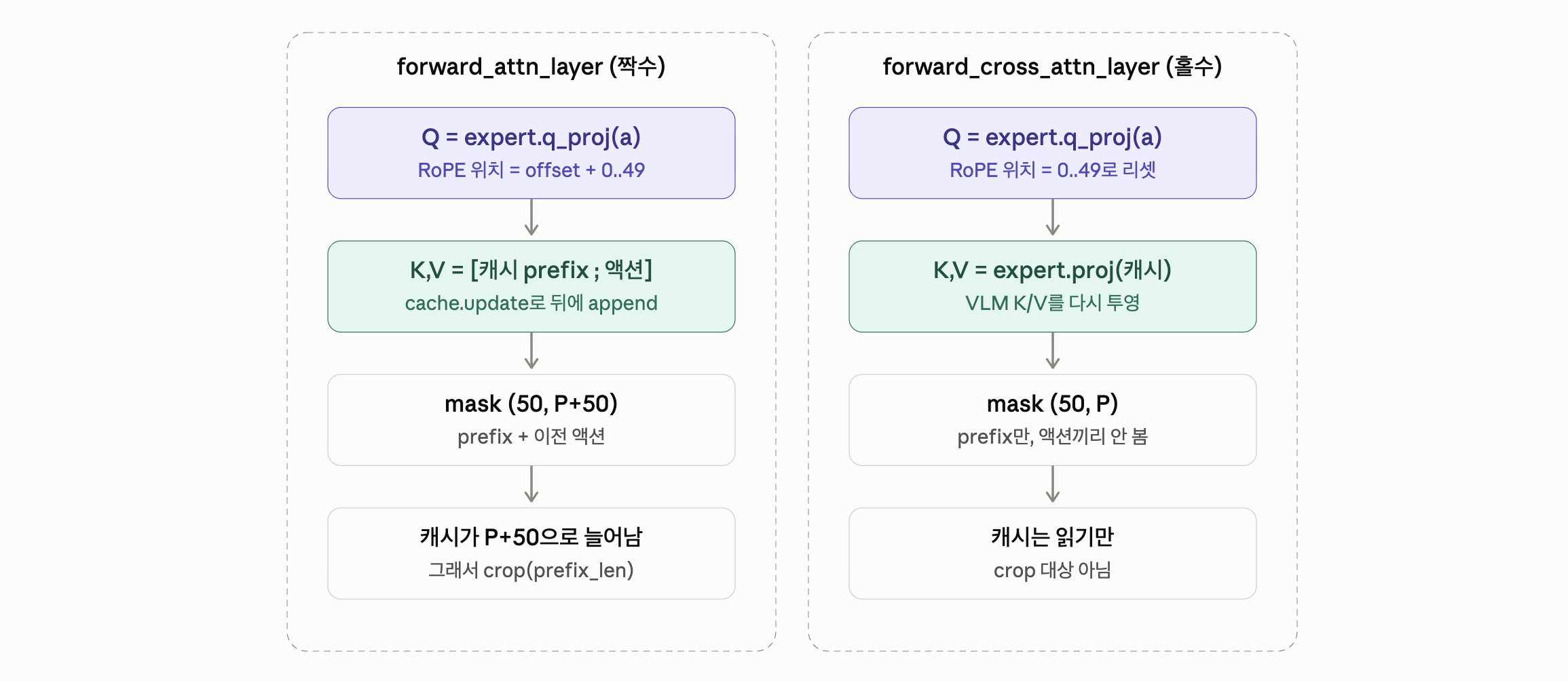
Forward_attn_layer (for EVEN LAYER)
핵심: KV Cache(prefix)에 액션의 K, V도 더해준다.
입력
- model_layers : 모델이 지금 우리는 2개이니까 이거 레이어를 독립적으로 저장.
- inputs_embeds : 임베딩 벡터
- layer_idx : 전체중 몇번째 레이어 인지
- position_ids, attention_mask
- batch_size, head_dim, use_cache
출력 - 어텐션 결과랑 past key values.
[att_output], past_key_values
코드를 한줄씩 다 읽어보자.
1
2
3
4
5
6
7
8
9
10
11
12
13
14
15
16
17
18
19
20
21
22
23
24
25
26
27
28
29
30
31
32
33
34
35

def forward_attn_layer(
    self, model_layers, inputs_embeds, layer_idx, position_ids,
    attention_mask, batch_size, head_dim, use_cache: bool = True,
    past_key_values: "DynamicCache | None" = None,
) -> "tuple[list[torch.Tensor], DynamicCache | None]":

    query_states = []
    key_states = []
    value_states = []

    for i, hidden_states in enumerate(inputs_embeds):
        layer = model_layers[i][layer_idx]
        if hidden_states is None or layer is None:
            continue

        # input layer norm을 먼저 진행시킴 RMSNorm 임.
        # (B, 50, 720), 960(prefix) 이 아니라 720(suffix) 이다.
        hidden_states = layer.input_layernorm(hidden_states)
        input_shape = hidden_states.shape[:-1]

        # 이게 그러니까 Head_dim = 64로 전부 고정이고, -1은 그러니까 유도리있게 바뀌도록
        hidden_shape = (*input_shape, -1, layer.self_attn.head_dim)

        hidden_states = hidden_states.to(dtype=layer.self_attn.q_proj.weight.dtype)

        # Query, key value 실제 연산이 일어남.
        # 여기서 K, V 는 Action hidden state 로부터임.
        query_state = layer.self_attn.q_proj(hidden_states).view(hidden_shape)
        key_state = layer.self_attn.k_proj(hidden_states).view(hidden_shape)
        value_state = layer.self_attn.v_proj(hidden_states).view(hidden_shape)

        query_states.append(query_state)
        key_states.append(key_state)
        value_states.append(value_state)
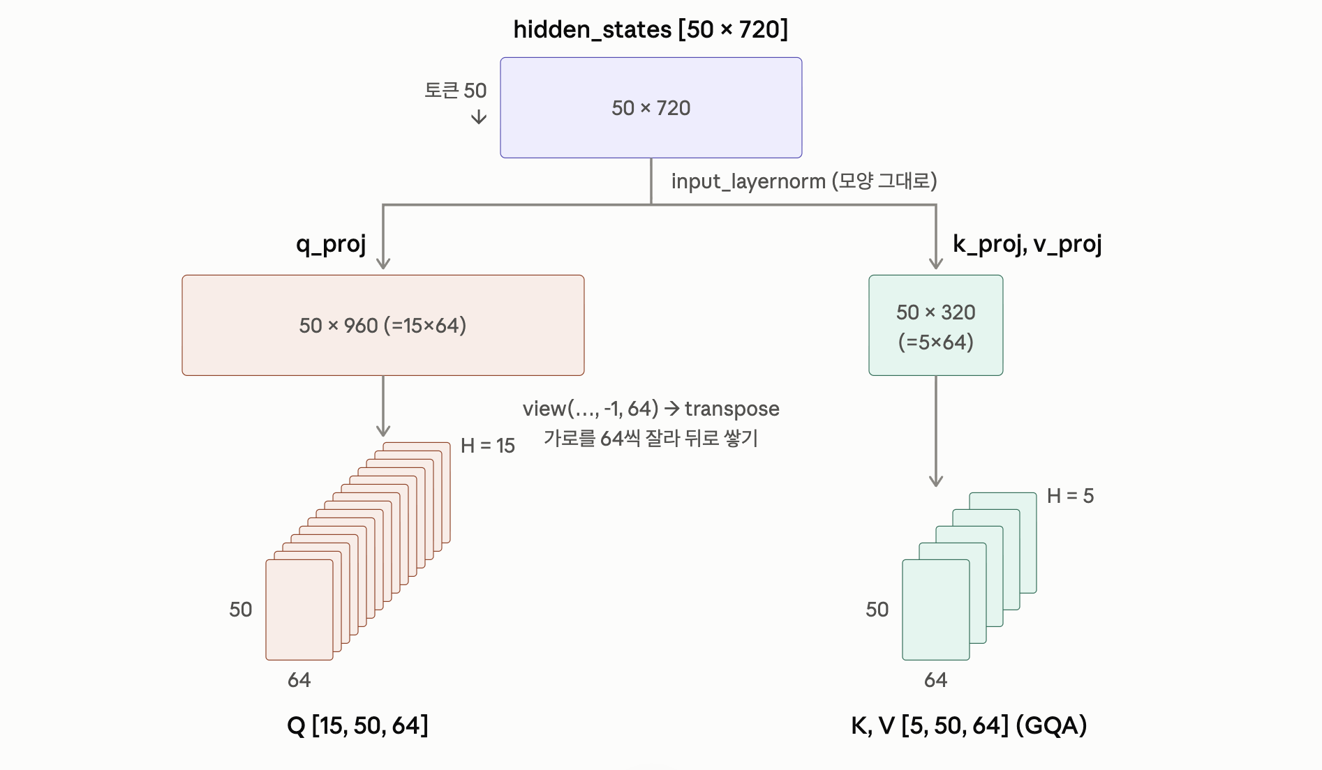
여기서 중요한 점은 바로,
- hidden states = embedding vector 이라는 것을 인지해야한다.
- 그리고 여기서 이제 head_dim에 맞게 shape을 바꿔주는게 핵심이다.
- 진짜 진짜 중요한거는 결국 지금 구한 key, value는 Action token 임베딩으로부터 도출된것!!!
- 즉 이 K, V를 우리가 미리 구한 Prefix K, V 뒤에 이어붙인다. (아래 past_key_values.update)
여기서 재미있는게 이제 Q,K,V는 prefix suffix 같이 일어나니까
Q - 960 , K,V - 320 으로 맞춰준다.
이후 코드를 같이 살펴보자,
1
2
3
4
5
6
7
8
9
10
11
12
13
14
15
16
17
18
19
def forward_attn_layer(
    self, model_layers, inputs_embeds, layer_idx, position_ids,
    attention_mask, batch_size, head_dim, use_cache: bool = True,
    past_key_values: "DynamicCache | None" = None,
) -> "tuple[list[torch.Tensor], DynamicCache | None]":

    ...

    # B,L,H,D with L sequence length, H number of heads, D head dim
    # concatenate on the number of embeddings/tokens
    query_states = torch.cat(query_states, dim=1)
    key_states = torch.cat(key_states, dim=1)
    value_states = torch.cat(value_states, dim=1)
    seq_len = query_states.shape[1]

    # RoPE는 지난시간에 다루었듯이, 회전한 정도를 우리가 위치 벡터로 정의한다면,
    # 같은 회전정도를 같은 위치라고 상대적으로 인지할 수 있다.
    query_states = apply_rope(query_states, position_ids_)
    key_states = apply_rope(key_states, position_ids_)
위에서 Concat 으로 이제 모든 query, key, value를 합치고 q,k에 대해서만 RoPE로 위치 벡터를 적용시켜주자, 이제 이후에 attention 과정에 들어가게 된다. !!!이제 여기서 아주 중요한게, K,V cache를 Prefix + Action을 더해주는 과정이 필요하다는 것.
1
2
3
4
5
6
7
8
9
...

 if use_cache:
     key_states, value_states = past_key_values.update(
         key_states.transpose(1, 2),
         value_states.transpose(1, 2), layer_idx
     )
     key_states = key_states.transpose(1, 2)
     value_states = value_states.transpose(1, 2)
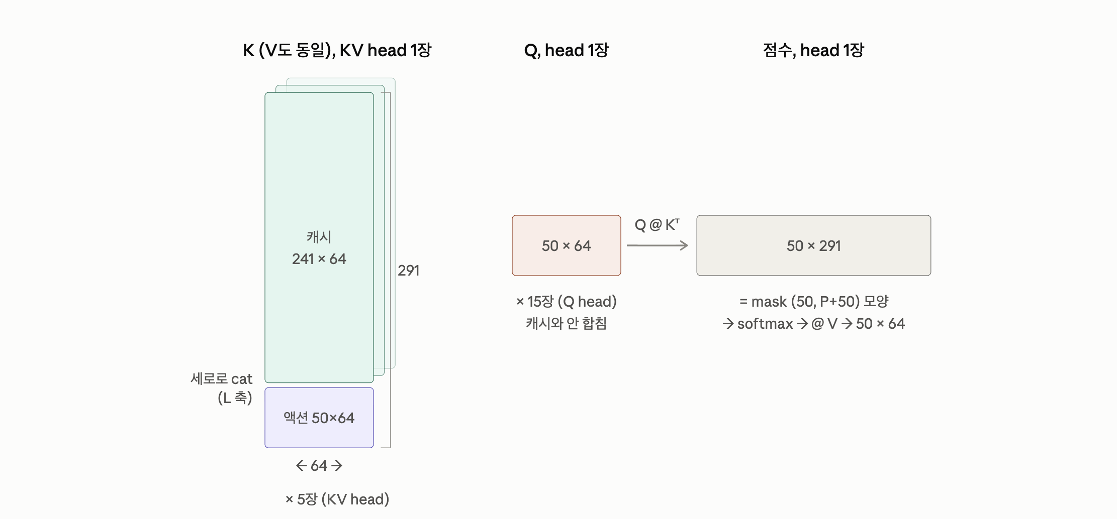
우리가 다루었듯이 저장되는 KV Cache from prefix 의 디멘션은 다음과 같다.
[B = 1, H = 5 , L_p = 241, D_H = 64 ]
1
2
3
4
5
6
7
# Prefix 에서 저장한 KV Cache
past_key_values (DynamicCache)
 ├─ layers[0]  : keys [1, 5, 241, 64], values [1, 5, 241, 64]
 ├─ layers[1]  : keys [1, 5, 241, 64], values [1, 5, 241, 64]
 │   ...
 └─ layers[15] : keys [1, 5, 241, 64], values [1, 5, 241, 64]
                       B  H   L   D
그리고 마지막으로 eager_attention_forward 메서드 안에 이제 우리가 아는 어텐션 아웃풋값을 구하는 코드가 최종적으로 들어있다. (지난시간에 다루었기 때문에 여기서는 넘어가자)
최종적으로 output은 그래서 2가지이다. 여기서 attention output의 디멘션은 바로 - [B = 1, L = 50, 960]
1
return [att_output], past_key_values
정리를 해보면, 결국에 아주 간략하게 정리를 하면,
- q,k,v를 먼저 Action token embedding기준으로 제작한다.
- (action token embedding → k,v) + (prefix → k,v) = k_new, v_new
- q,k_new, v_new 를 가지고 attention 연산을 진행.
- [att_output] 저장
Forward_cross_attn_layer (for ODD LAYER)
그 다음 이제 대망의 cross attention을 살펴보자. self attention 과 거의 비슷하지만 한가지만 다르다.
바로, K , V cache prefix only를 그대로 사용한다는 점이다.
여기서, 먼저 가중치와 곱하기 위해서 디멘션을 바꾸고 가중치를 곱한다음에 그리고 다시 원래로 복귀.
1
2
3
4
5
6
7
8
9
10
11
12
13
14
15
16
17
18
19
20
21
22
23
24
25
26
def forward_cross_attn_layer(

    attention_interface = self.get_attention_interface()

    att_outputs = []
    assert len(inputs_embeds) == 2 or (use_cache and past_key_values is not None), (
        f"Both len(inputs_embeds) == {len(inputs_embeds)} and past_key_values is {past_key_values}"
    )

    ...

        # reshape (not view): K/V read back from the cache are transposed, hence non-contiguous
        _key_states = key_states.to(dtype=expert_layer.self_attn.k_proj.weight.dtype).reshape(
            *key_states.shape[:2], -1
        )
        expert_key_states = expert_layer.self_attn.k_proj(_key_states).view(
            *_key_states.shape[:-1], -1, expert_layer.self_attn.head_dim
        )  # k_proj should have same dim as kv

        _value_states = value_states.to(dtype=expert_layer.self_attn.v_proj.weight.dtype).reshape(
            *value_states.shape[:2], -1
        )
        expert_value_states = expert_layer.self_attn.v_proj(_value_states).view(
            *_value_states.shape[:-1], -1, expert_layer.self_attn.head_dim
        )
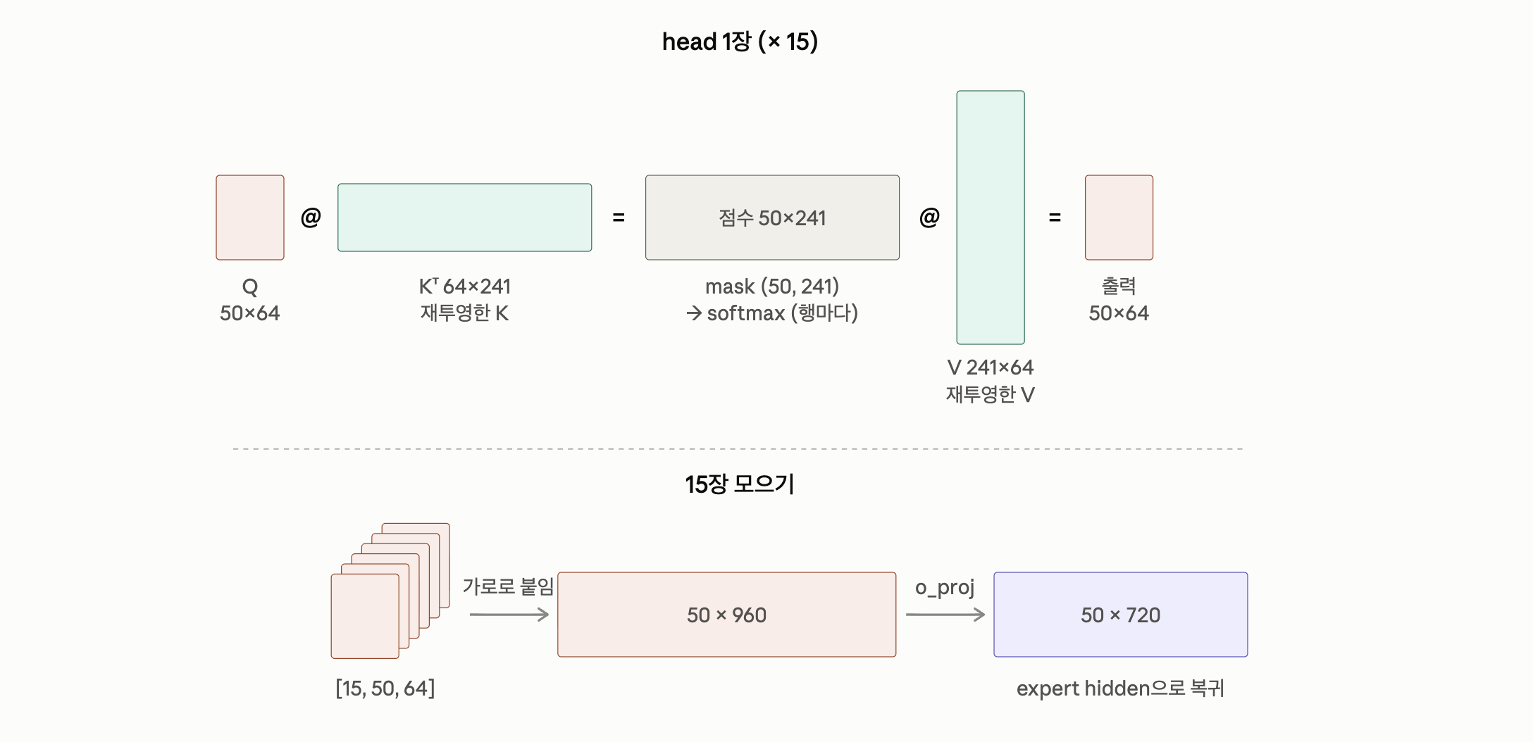
결국에 사실 291 → 241길이의 K, V 를 가지고 진행하는 것이라고 이해하면 된다. 사실 이전 이랑 크게 다를 것이 없다.
여기서 이제 attention 연산을 진행하기 앞서서 Query부분에만 이제 position id 를 적용해준다. 실제로 여기서 Query만 시간과 노이즈로 결정되는 입력 변수이므로, 우리는 위치정보를 더해주는 것이다.
1
2
3
4
5
6
7
8
expert_position_id = (
    expert_position_id - torch.min(expert_position_id, dim=1, keepdim=True).values
)  # start from 0
expert_attention_mask = attention_mask[
    :, -inputs_embeds[1].shape[1] :, : expert_key_states.shape[1] :
]  # take into account kv

expert_query_states = apply_rope(expert_query_state, expert_position_id)
여기서 3가지가 처음 보면 좀 이상한데, 이유는 사실 하나다.
cross 층에서는 prefix(캐시 K)와 액션(Q)의 좌표축이 끊겨 있다
캐시의 prefix K는 RoPE로 회전된 다음, expert의 k_proj(Linear)가 320차원을 통째로 섞어버린다. 그래서 RoPE 회전 구조가 깨지고, prefix랑 액션이 같은 좌표축에 있지 않게 된다.
1) position id - min → 0부터 다시 세기
offset + 0..49→0..49. 좌표축이 끊겼으니 prefix 뒤에 이어 붙일 이유가 없다. 오히려 offset은 프롬프트 길이마다 달라서 남겨두면 잡음이 된다.
2) mask 자르기 → prefix 열만 남기기
attention_mask[:, -50:, :P]→(B, 50, P+50)→(B, 50, P)
cross 층은 K/V가 prefix P개뿐이니까 열도 앞 P개면 충분하다. 이 층에서 액션끼리는 서로 안 본다.
3) RoPE는 Q에만 → “i번째 액션” 태그
K는 이미 회전된 걸 재투영한 거라 다시 안 돌린다. Q만 돌리면 상대 위치는 아니지만, i번째 액션마다 prefix를 다른 각도로 보게 된다 → 절대 위치 태그 역할.
정리하면,
- self 층: 한 좌표축 → offset 이어붙이기 + Q, K 둘 다 RoPE (상대 위치)
- cross 층: 좌표축 끊김 → offset 제거 + prefix 열만 + Q만 RoPE (절대 위치 태그)
이제 Forward에서 우리는 지금까지 복잡한 어텐션 연산 쪽을 쭉 go over했고, 이제 attention으로 얻은 outputs embedding vector을 가지고 사실 projection layernorm 작업을 진행해줘야한다.
1
2
3
4
5
6
7
8
9
10
11
12
13
14
15
16
17
18
19
20
21
22
23
24
25
26
27
28
29
30
31
32
33
34
35
36
37
38
39
40
41
42
43
44
45
#(def forward 이어서)

         outputs_embeds = []
         start = 0
         for i, hidden_states in enumerate(inputs_embeds):
             layer = model_layers[i][layer_idx]
             att_output = (
                 att_outputs[i] if i < len(att_outputs) else att_outputs[0]
             )  # in case of self_attn
             if hidden_states is not None:
                 if layer is None:
                     outputs_embeds.append(hidden_states)
                     continue
                 end = start + hidden_states.shape[1]

                 if att_output.dtype != layer.self_attn.o_proj.weight.dtype:
                     att_output = att_output.to(layer.self_attn.o_proj.weight.dtype)
                 att_out = att_output[:, start:end]
                 out_emb = layer.self_attn.o_proj(att_out)

                 out_emb += hidden_states
                 after_first_residual = out_emb.clone()

                 out_emb = layer.post_attention_layernorm(out_emb)
                 out_emb = layer.mlp(out_emb)

                 out_emb += after_first_residual

                 outputs_embeds.append(out_emb)

                 start = end if len(att_outputs) == 1 else 0
             else:
                 outputs_embeds.append(None)

         inputs_embeds = outputs_embeds

     # final norm
     outputs_embeds = []
     for i, hidden_states in enumerate(inputs_embeds):
         if hidden_states is not None:
             out_emb = models[i].norm(hidden_states)
             outputs_embeds.append(out_emb)
         else:
             outputs_embeds.append(None)
     return outputs_embeds, past_key_values
D. Action Projection
이제 우리가 얻은 output_embeds → velocity로 결국 최종적으로 도출하는 것이 목표이고, 이제 이 작업은 그냥 사실상 프로젝션 과정으로 진행하면 된다.
1
2
3
4
5
6
7
8
9
10
11
12
13
14
15
16
17
18
19
20
21
22
23
## lerobot -> policies -> smolvla -> modeling_smolvla.py

def denoise_step(
    self,
    prefix_pad_masks,
    past_key_values,
    x_t,
    timestep,
):
    """Apply one denoising step of the noise `x_t` at a given timestep."""

    ...

    # D - Projection
    if past_key_values is not None:
        # Self-attention layers append suffix K/V in place; restore the prefix for the next step.
        past_key_values.crop(prefix_len)
    suffix_out = outputs_embeds[1]
    suffix_out = suffix_out[:, -self.config.chunk_size :]
    suffix_out = suffix_out.to(dtype=torch.float32)
    v_t = self.action_out_proj(suffix_out)
    return v_t
4. After denoising loop x 10
먼길을 왔지만 인셉션 처럼 우리는 사실 디노이징 루프를 돌고 있었다. ㅋㅋㅋ 저 루프를 10번 돈다음에 이제 돌아오면 우리가 원하는 x_t 즉 로봇 관절값이 도출된다.
1
2
3
4
5
6
7
8
9
10
11
12
13
14
15
16
17
18
19
20
21
22
23
24
25
26
27
28
###############################################################
########## Next step euler_integrate and denoise_step #########
###############################################################

torch.manual_seed(0)

num_steps = model.config.num_steps # 10 in here
dt = -1.0 / num_steps              # -0.1 (t changes from 1 -> 0)

x_t = noise
with torch.no_grad():
    for step in range(num_steps):
        t = 1.0 + step * dt
        time_tensor = torch.full((bsize,), t , dtype = torch.float32)

        v_t = model.denoise_step(
            prefix_pad_masks = prefix_pad_masks,
            past_key_values = past_key_values,
            x_t = x_t,
            timestep = time_tensor
        )

        x_t = x_t + dt * v_t # Euler one step

        print(f"step {step} t={t:.1f} v_t {tuple(v_t.shape)} "
              f"cache_len {past_key_values.get_seq_length()}")
마지막 최종 단계 후처리: unpad → 역정규화
Euler 10 step이 끝난 $x_0$ [1, 50, 32]는 아직 정규화 공간의 값이다. 로봇에 보내려면 두 단계를 거친다.
- unpad:
x_0[:, :, :6]→[1, 50, 6](32칸 중 SO-101 6 DOF만 진짜, 나머지는 패딩) - 역정규화:
post(actions)→ $a_{real} = a_{norm} \cdot \sigma + \mu$
1
2
actions_norm = x_t[:, :, :6]        # unpad
actions_real = post(actions_norm)   # 역정규화
여기서 우리가 필요한 건 관절마다 2개 (mean, std).
(단, action용과 state용이 따로 있다 (SO-101이면 각각 6 + 6))
- 이 값은 학습으로 얻는 게 아니라, 데이터셋 녹화 시
meta/stats.json에 자동 계산→ fine-tuning 체크포인트에 같이 저장된다. 그래서 학습 때와 같은 로봇 · 같은 셋업으로 추론해야 함.
- action / state가 따로인 이유:
observation.state는 로봇이 지금 있는 각도(follower, 입력),action은 가라고 명령한 목표 각도(leader, 출력)라 분포가 미묘하게 다르다 → feature 키마다 따로 계산.
Summary
최종적으로 디멘션을 중심으로 어떻게 우리가 관절값을 얻는지 한눈에 봐보자.
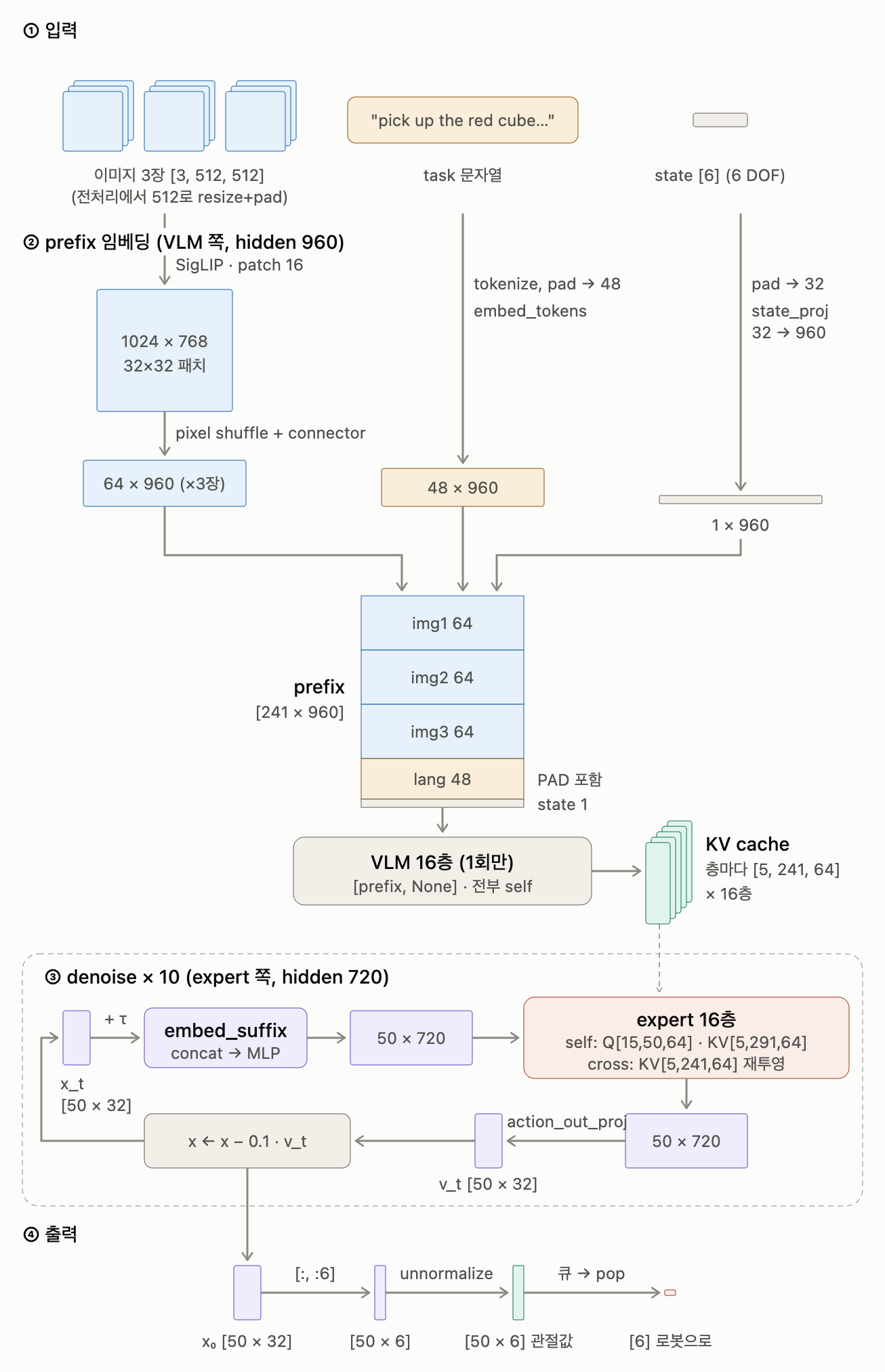
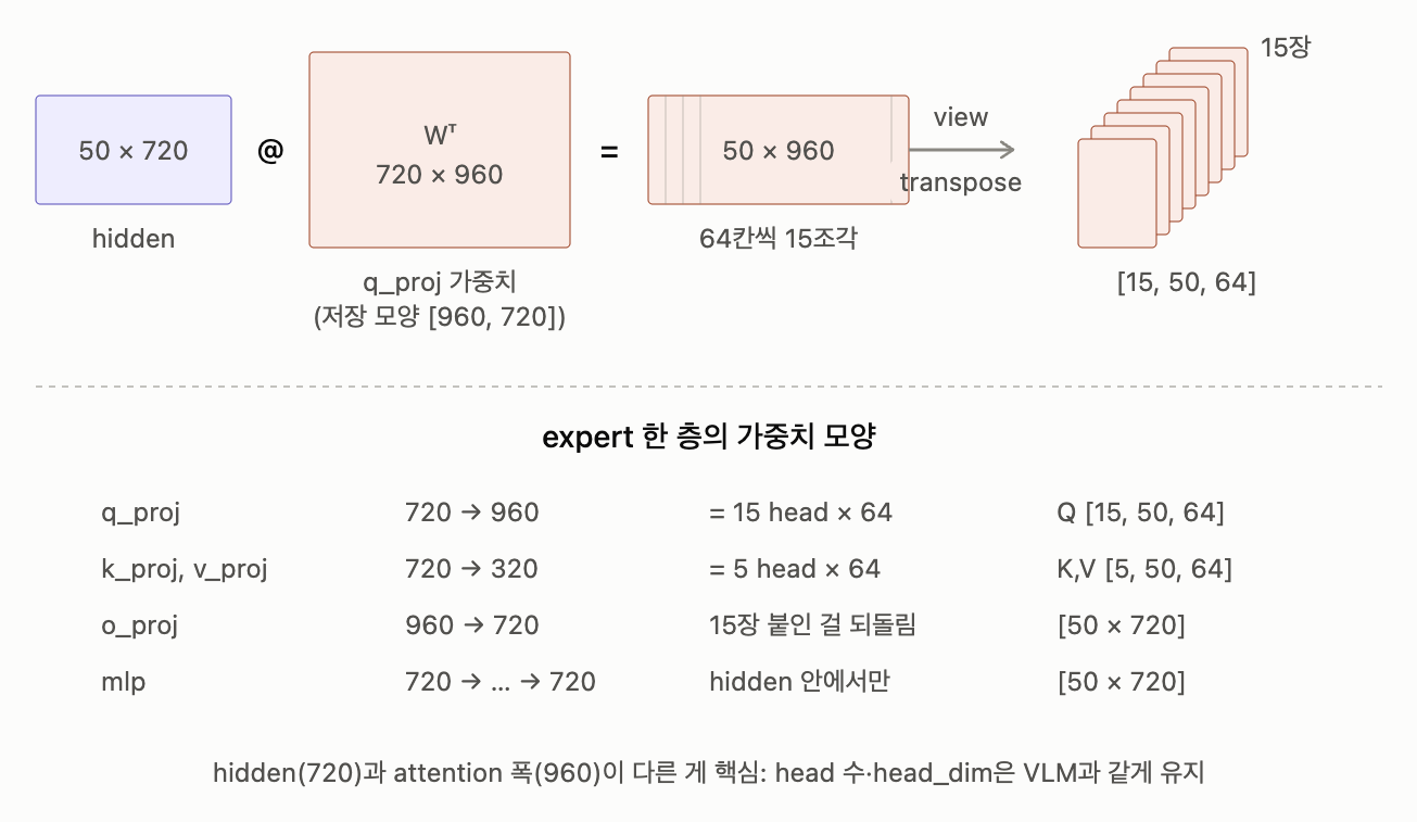
Attention Weight
어텐션의 가중치(W_q)가 결국에 suffix(720) and prefix(960) Embedding → 960차원(15 head × 64)으로 맞춰주는 역할을 진행한다. (K, V는 320차원 = 5 head × 64, GQA) → 그래서 입력 차원이 달라도 같은 attention 연산을 할 수 있는 것.