π₀ - Vision-Language-Action Flow Model
π₀는 PaliGemma VLM에 Action Expert를 어떻게 붙였고, Gaussian noise에서 continuous action chunk를 어떻게 만들어낼까? attention mask, flow matching, loss function을 하나씩 짚어봤다.
논문: 𝜋_0: A Vision-Language-Action Flow Model for General Robot Control
Date 2024.10.31
Architecture
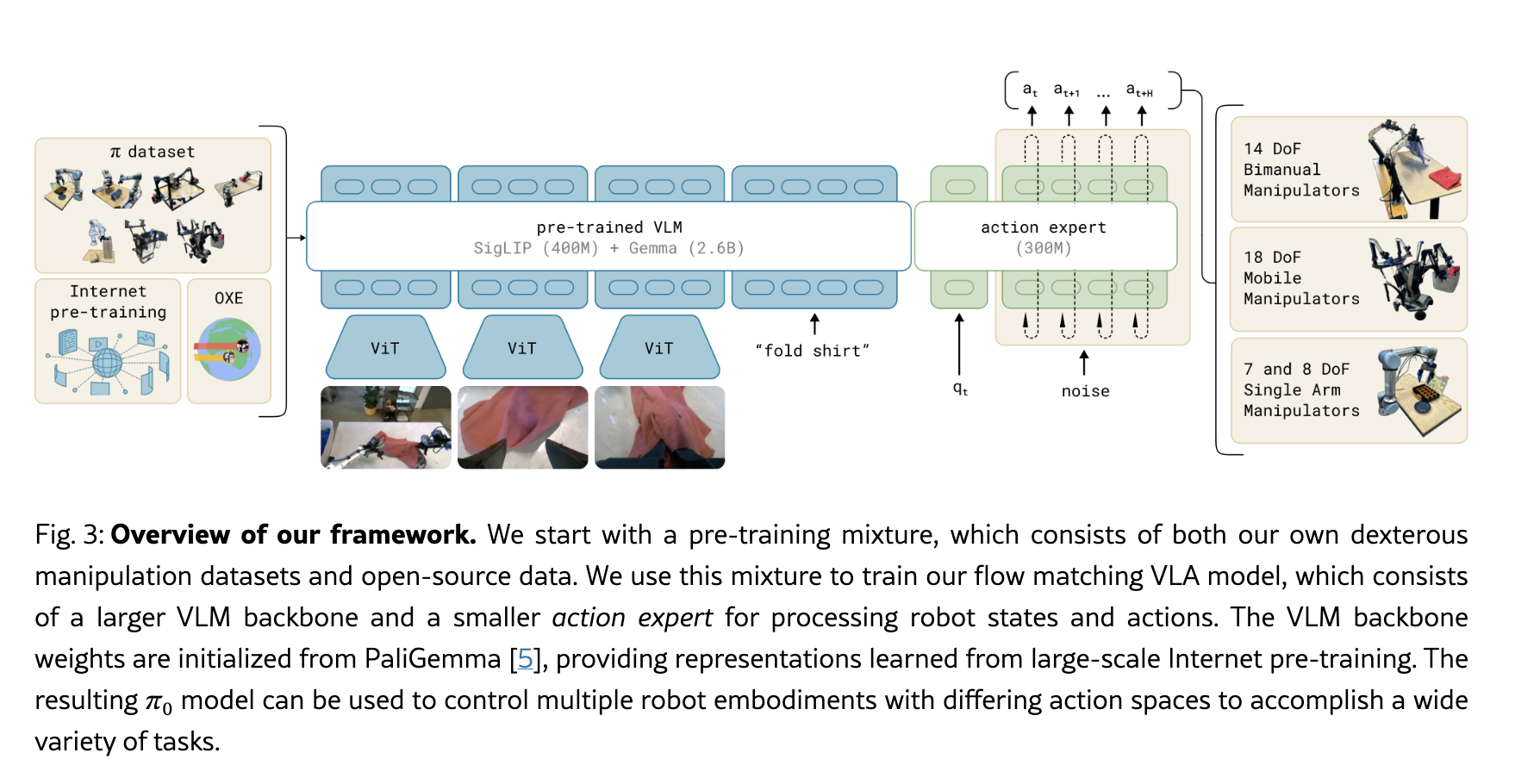
차별점 vs RT2 (google deepmind)
- RT-2: pretrained VLM을 web vision-language data + robot trajectory data로 co-fine-tuning하고, robot action을 discrete language-like tokens로 autoregressive하게 생성한다.
- π0: pretrained VLM(PaliGemma)에 별도의 Action Expert (~300M)를 추가하고, continuous action을 Flow Matching으로 생성한다.
- 단순히
VLM → Action Expert로 직렬 연결된 두 network가 아니다. - Image/Text token은 PaliGemma expert의 weights를, State/Noisy Action token은 Action Expert의 weights를 사용하면서 attention layer에서 서로 representation을 교환한다.
- 따라서 π0의 핵심 architecture는
VLM semantic expert ↔ shared attention ↔ Action Expert로 이해하는 것이 좋다.
- 단순히
- Input을 보면 Image + instruction(text)에 더해 robot state
q_t(proprioception)가 명시적으로 들어간다.- Image → 외부 환경에서 무엇을 보고 있는가?
- Language instruction → 무엇을 해야 하는가?
- State
q_t→ 현재 robot body가 어떤 상태인가? (joint angle 등 proprioception) - Noisy Action → 현재 Flow Matching 과정에서 clean action으로 변환해야 하는 action sample
- 즉 observation은 대략
o_t = [images, language, q_t]이고, state와 noisy action은 Action Expert 쪽 token으로 들어간다. - output is not just single action but the action chunk
기존에는 RT2의 경우에는 아래처럼 8개의 토큰을 하나의 action으로 output 하였다.

- 하지만 π0는 Action Chunk를 사용한다. 즉 한 시점의 action 하나가 아니라 미래의 여러 action을 묶어서 한 번에 생성한다. 논문 설정에서는
H = 50, 즉A_t = [a_t, a_{t+1}, ..., a_{t+49}]. - 중요: Action Chunk와 Flow Matching은 서로 다른 개념이다.
- Action Chunk = 미래 여러 timestep의 robot action을 한 번에 출력하는 것.
- Flow Matching = Gaussian noise로 시작한 action sample을 clean action chunk distribution으로 이동시키는 vector field를 학습하는 생성 방법.
- 따라서 여기서
flow는 실제 로봇이 시간에 따라 움직이는 trajectory의 흐름을 뜻하는 것이 아니다.
- Inference에서는 대략
Noise Action → Flow velocity prediction → Euler integration 반복 → Clean Continuous Action Chunk순서로 생성된다. π0에서는 10 Euler integration steps를 사용한다. ( Diffusion image model 과 동일한 원리이다)
- VLM은 robot data만으로 처음부터 학습한 모델이 아니라, 기존의 PaliGemma pretrained VLM을 사용한다. 따라서 web-scale vision-language pretraining에서 얻은 semantic/world knowledge를 robot control에 활용할 수 있다.
π0 Architecture 핵심 요약
- Total parameters: 약 3.3B
- VLM backbone: PaliGemma 3B (SigLIP vision encoder + Gemma language model)
- Action Expert: 약 300M, scratch initialization
- Robot state: proprioception
q_t를 명시적으로 conditioning - Action horizon:
H = 50action chunk - Action generation: Conditional Flow Matching
- Inference: Gaussian noise → learned vector field → 약 10-step Euler integration → continuous action chunk
RT-2 → π0의 핵심 진화:
Discrete Action Tokens→Separate Action Expert + Continuous Flow Matching + Action Chunk. 즉, VLM의 semantic knowledge는 유지하면서 motor control을 위한 별도의 continuous generative policy를 붙였다는 것이 핵심이다.
세가지를 코드에서 직접 보고 들어가자. 직접 코드를 읽으면서 세부사항들을 짚고 넘어가자.
Q1. Cross attention vs self Attention , prefix → action으로 어떻게 넘어가는거지?
여기서 input token을 다음과 같이 하나로 표현하자.

token을 임베딩에 넣어서 각 토큰을 벡터로 바꿔주면 아래와 같은 Matrix이 도출된다.
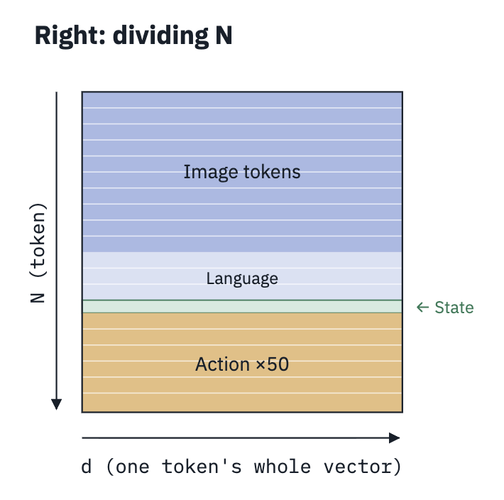
전체 아키텍쳐는 다음과 같다. 여기서 최종 output token에서 뒷부분 action부분만 보는 것이다.
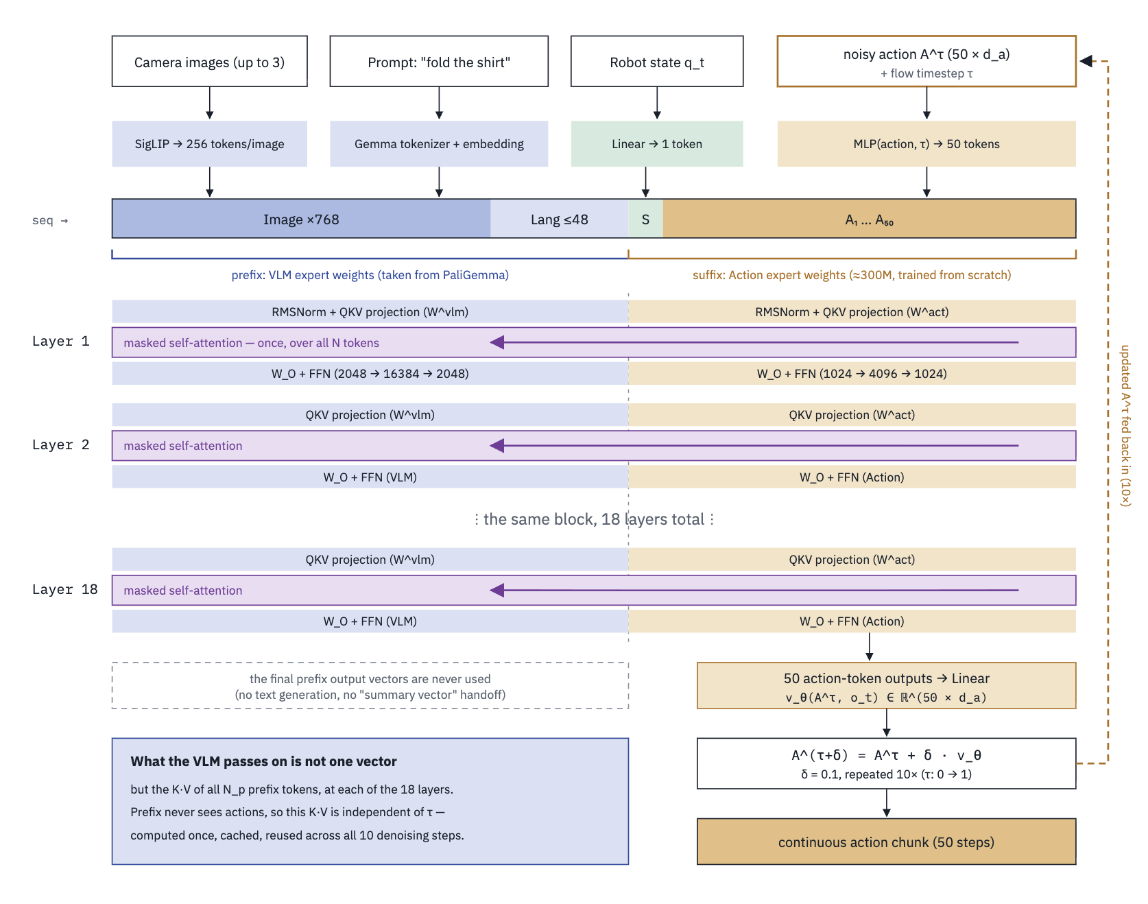
사실 Masked self - attention 부분이 핵심인데, 이 부분을 자세하게 봐보자. 이부분이 정말 재미있다. 나는 당연히 cross attention으로 K,V에다가 prefix token을 넣고, Q에다가 Action token을 당연히 넣을꺼라고 생각했는데, 그게 아니었다. 가중치를 그냥 VLM(PaliGemma) expert + Action을 합치는 기가막힌 마술을 하였다. 다음과 같다.
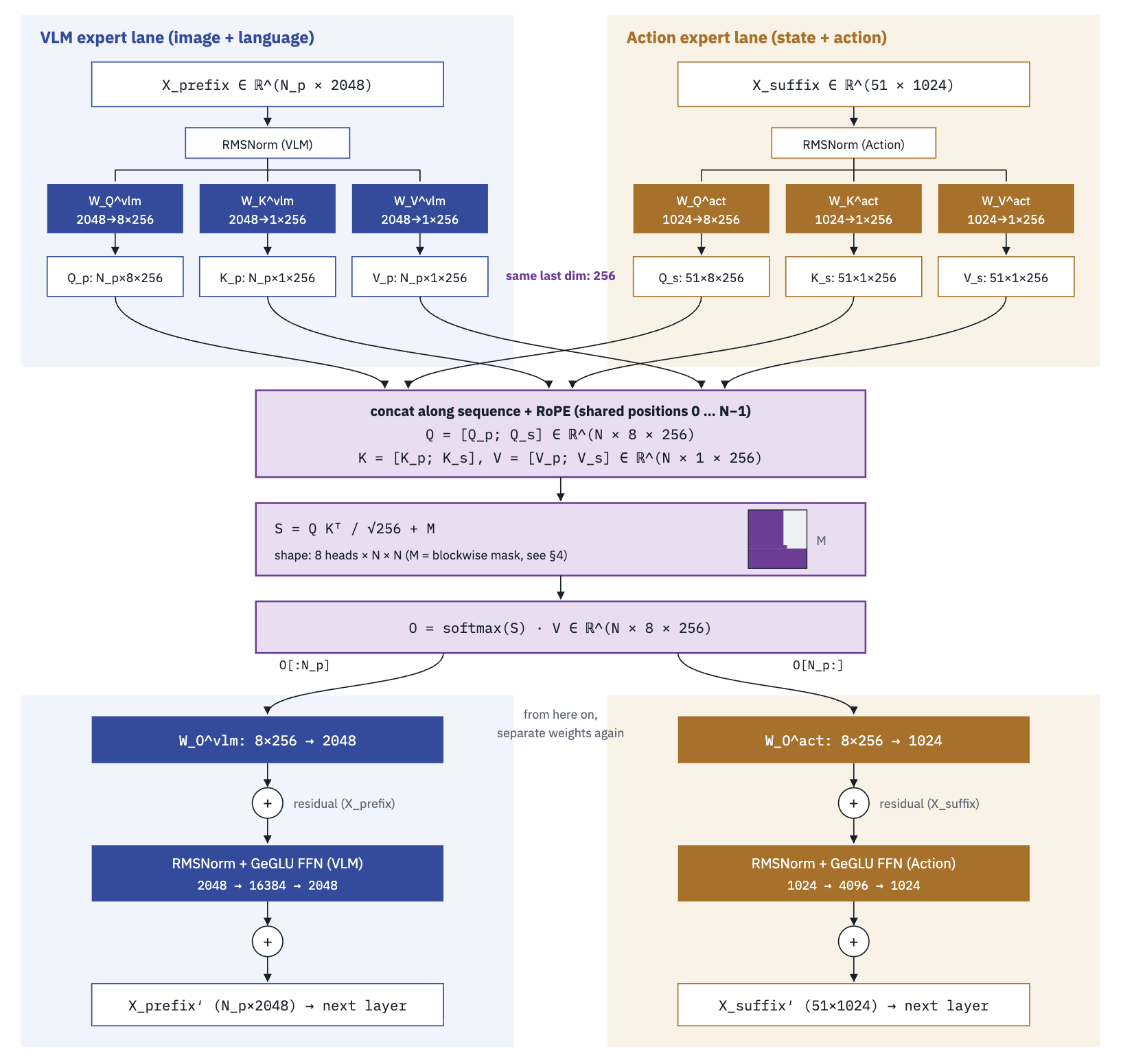
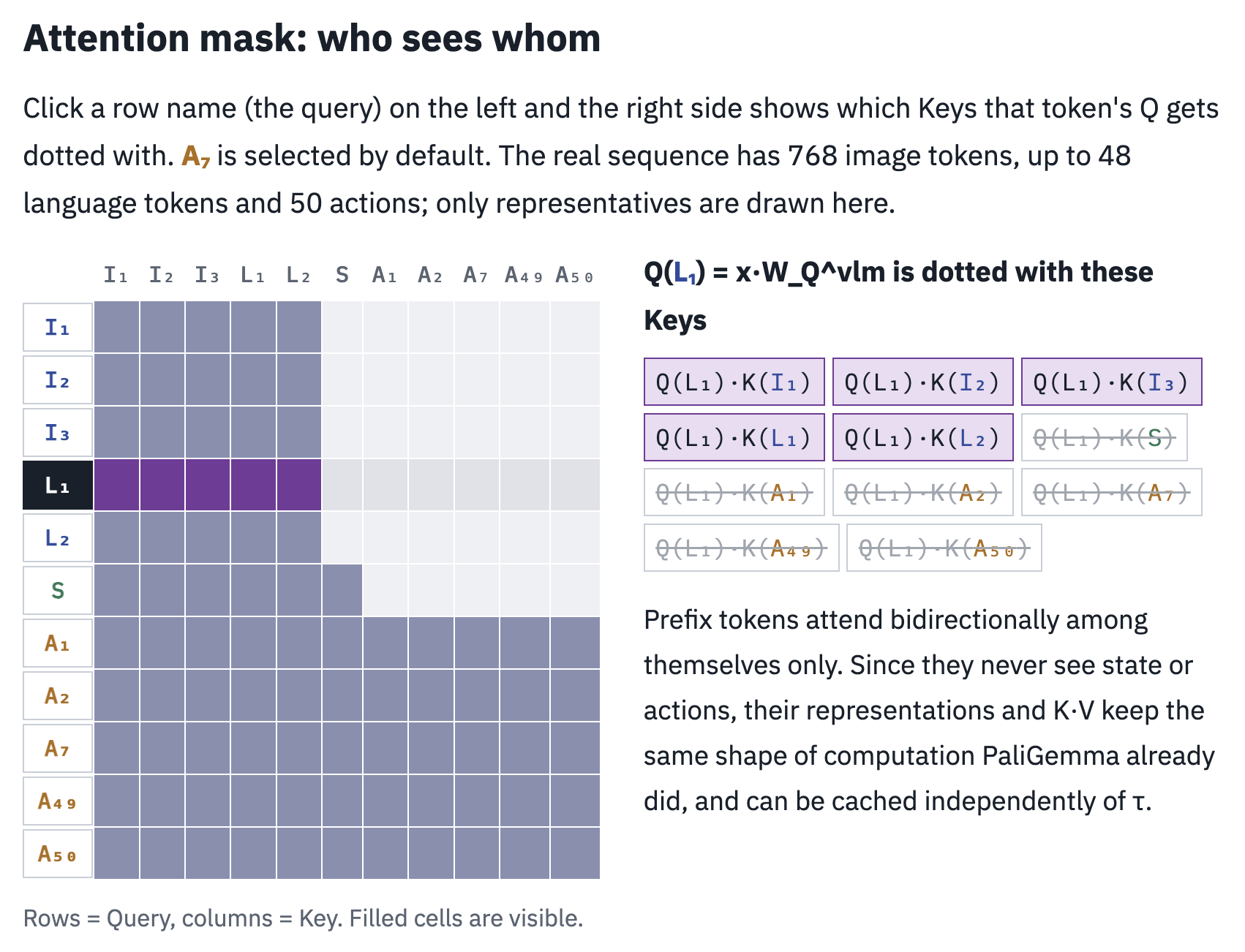
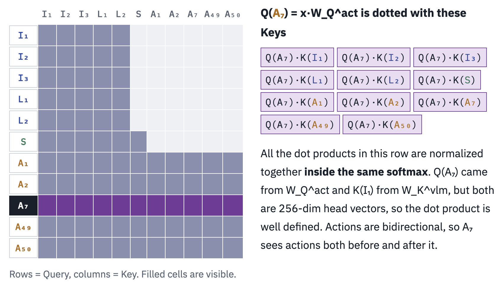
여기서 Self Mask 부분이 가장 중요한데, 결국에 VLM(PaliGemma) expert의 가중치는 이미지와 텍스트 즉 prefix 토큰 끼리만 양방향으로 보도록 S, A 토큰들은 전부 마스크 해준다. 그리고, 오히려 State는 Prefix + State 그리고, Action은 모두다 참고하도록 설계를 진행하였다. 이게 재미있는 부분이다.
Q2. Noise → action 부분 정확히 어떤 식으로 구현이 되는건지 궁금
π0는 action을 직접 한 번에 예측하지 않고, Gaussian noise에서 실제 action distribution으로 이동시키는 velocity field를 학습한다. 이 방식이 Conditional Flow Matching이다. (아래의 이미지 diffusion model과 같은 원리이다)
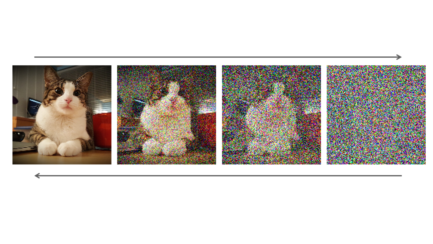
먼저 실제 demonstration에서 action chunk를 가져온다.
\[A_t = [a_t, a_{t+1}, \cdots, a_{t+H-1}]\]π0에서는 action horizon이
\[H = 50\]이므로, 한 번에 미래 50개의 action을 생성한다. (Action1 → …. → Action 50 으로 목표달성) 그 다음 동일한 dimension의 Gaussian noise를 sampling한다.
\[\epsilon \sim \mathcal{N}(0,I)\]Noise와 실제 action chunk 사이의 중간 상태를 다음과 같이 만든다.
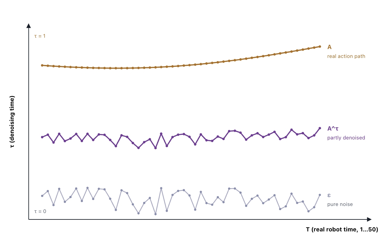
\[A_t^\tau = \tau A_t + (1-\tau)\epsilon\]여기서 $\tau \in [0,1]$는 실제 robot time이 아니라 flow interpolation time이다.
\[\tau=0 \Rightarrow A_t^\tau = \epsilon\] \[\tau=1 \Rightarrow A_t^\tau = A_t\]즉 $\tau$가 증가하면서
\[\text{Noise} \rightarrow \text{Action}\]으로 이동한다.
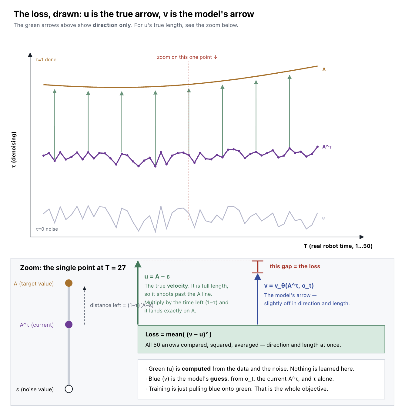
아래 그래프를 보면 이해가 쉽다. 즉 아래에서 위로 디노이징이 되고, 각각 실제 시간 T에 대해서 왼쪽에서 오른쪽으로 로봇이 액션하는 movement라고 이해하면 쉽다.
직선 보간을 사용했으므로 이 경로의 정답 velocity는
\[A_t^\tau = \tau A_t + (1-\tau)\epsilon\] \[u(A_t^\tau \mid A_t) = \frac{dA_t^\tau}{d\tau} = A_t-\epsilon\]가 된다. Action Expert는 현재 noisy action $A_t^\tau$와 observation $o_t$를 입력받고
\[v_\theta(A_t^\tau,o_t)\]를 출력한다. 이 값은 단순한 방향만이 아니라, 각 action dimension을 어느 방향으로 얼마나 빠르게 변화시켜야 하는지를 나타내는 velocity vector이다.
부호 주의: 논문(arXiv v1~v3) 본문은 위와 똑같이 $A_t^\tau = \tau A_t + (1-\tau)\epsilon$으로 정의해 놓고 target을 $u = \epsilon - A_t$로 적어 놨다. 그런데 직접 미분해보면 $A_t - \epsilon$이 맞고, 실제로 v4(2026.01)에서는 $A_t - \epsilon$으로 고쳐져 있다.
반대로 openpi 코드(
pi0.py)는 diffusion 쪽 관례대로 τ 방향을 거꾸로 잡는다.x_t = t * noise + (1 - t) * actions(t=1이 noise, t=0이 action)라서 target이u_t = noise - actions, 즉 $\epsilon - A_t$가 되고, sampling도 t를 1→0으로dt = -1/num_steps씩 적분한다.결국 τ 축을 뒤집었을 뿐 같은 것이다. 코드 볼 때 부호 때문에 햇갈리지 말자.
Inference에서는 noise에서 시작해 학습된 velocity field를 반복적으로 적분한다.
\[A^{\tau+\Delta\tau} = A^\tau + \Delta\tau\,v_\theta(A^\tau,o_t)\]즉 개념적으로
\[\epsilon \rightarrow A^{\tau_1} \rightarrow A^{\tau_2} \rightarrow \cdots \rightarrow A\]와 같이 Euler integration을 수행하여 최종 continuous action chunk를 얻는다.
핵심: Action Expert가 직접 정답 action을 출력하는 것이 아니라, 현재 noisy action을 clean action 쪽으로 이동시키는 velocity field를 출력한다.
Q3. 학습할때 Loss function을 정확하게 어떻게 정의를 했을까?
논문에서 flow matching loss는 다음과 같이 정의된다.
\[L^\tau(\theta) = \mathbb{E}_{p(A_t\mid o_t),\,q(A_t^\tau\mid A_t)} \left[ \left\| v_\theta(A_t^\tau,o_t) - u(A_t^\tau\mid A_t) \right\|^2 \right]\]각 항의 의미는 다음과 같다.
- $A_t$: dataset에서 가져온 실제 action chunk
- $o_t$: 현재 observation
- $A_t^\tau$: noise와 실제 action 사이의 중간 상태
- $v_\theta(A_t^\tau,o_t)$: Action Expert가 예측한 velocity
- $u(A_t^\tau\mid A_t)$: flow matching에서 정의된 ground-truth velocity
직선 interpolation을 사용하면 target velocity는
\[u(A_t^\tau\mid A_t)=A_t-\epsilon\]이므로, 학습은 결국
\[\boxed{ L^\tau(\theta) = \mathbb{E} \left[ \left\| v_\theta(A_t^\tau,o_t) -(A_t-\epsilon) \right\|^2 \right] }\]와 같은 velocity MSE regression으로 이해할 수 있다.
학습 과정은 다음과 같다.
- Dataset에서 $(o_t,A_t)$를 가져온다.
Gaussian noise를 sampling한다.
\[\epsilon\sim\mathcal{N}(0,I)\]- Random flow time $\tau$를 sampling한다.
중간 noisy action을 만든다.
\[A_t^\tau=\tau A_t+(1-\tau)\epsilon\]Action Expert가 velocity를 예측한다.
\[v_\theta(A_t^\tau,o_t)\]정답 velocity와의 MSE를 최소화한다.
\[v_\theta(A_t^\tau,o_t)\approx A_t-\epsilon\]
따라서 중요한 점은 action 자체의 MSE를 계산하는 것이 아니라, velocity의 MSE를 계산한다는 것이다.
한 문장 요약: Noise와 실제 action 사이에서 임의의 중간점을 뽑고, 그 위치에서 실제 action 쪽으로 가야 하는 velocity를 Action Expert가 맞히도록 학습한다.
$\tau$는 action chunk의 50개 robot timestep index가 아니라 flow interpolation time이다. 50개의 action timestep과 $\tau$는 서로 다른 축이다.