SmolVLA - Training

이제 실제 VLA 학습단계에 들어가보자.

데이터 - lerobot/svla_so101_pickplace

GPU - A40 VRAM 48GB

Model - SmolVLA

Contents

---

1. Data loading
2. Data Processing
3. 학습 파라메터 vs Freeze 파라메터
4. Training loop (batch 2, 20 step 연습)
5. Fine-tuning preprocessing
6. Fine-tuning result

1. Data loading

---

일단 lerobot 에서 hugging face에 올려놓은 데이터를 다운로드를 받자.

lerobot/svla_so101_pickplace · Datasets at Hugging Face

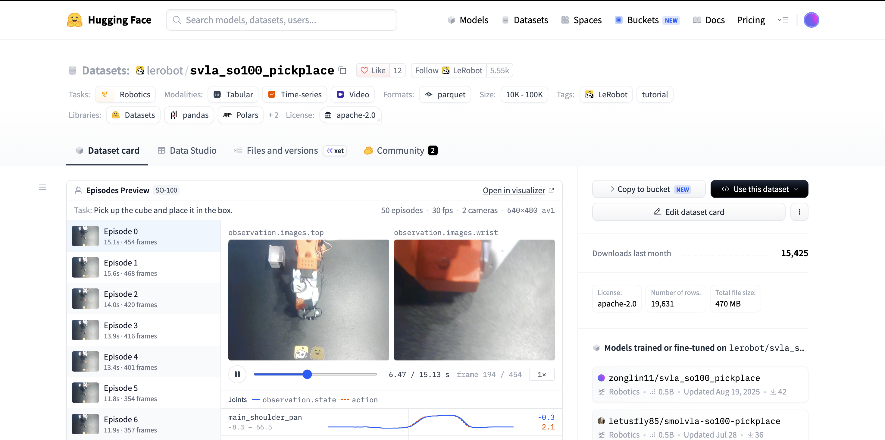
들어가보면, 로봇 공부를 위한 수많은 데이터들이 존재한다. 그리고 핵심은 이제 데이터가 굉장히 잘 정돈이 되어있는 상황이다.

바로 내 Local에서 데이터를 불러온다음에 그다음에 한번 열어서 어떻게 데이터 어떤 shape으로 저장되어있는지 확인하자.

# delta_timestamps: 현재 frame 부터 미래 50 step(30fps) action 을 묶어서 정답 chunk 로
from lerobot.datasets.lerobot_dataset import LeRobotDataset
ds = LeRobotDataset("lerobot/svla_so101_pickplace", root=DATA_DIR,
                    delta_timestamps={"action": [i / 30 for i in range(50)]})

실제 데이터에 담긴 정보를 output 해보면 다음과 같다.

print(len(ds), ds.meta.tasks)
x = ds[230]          # 전체 11939 frame 중 230 번째 frame 하나 꺼내기 (dict)
for k, v in x.items():
    print(k, getattr(v, "shape", v))

#Output
11939                                           task_index
task
pink lego brick into the transparent box           0

action torch.Size([50, 6])                  # delta_timestamps 덕분에 미래 50 step 정답 chunk
action_is_pad torch.Size([50])              # 에피소드 끝 넘어간 step 표시 (loss 에서 빠짐)
observation.state torch.Size([6])           # 현재 관절 위치 6개
observation.images.up torch.Size([3, 480, 640])     # 현재 카메라 사진 (mp4 에서 그때그때 디코딩)
observation.images.side torch.Size([3, 480, 640])
timestamp torch.Size([])
frame_index torch.Size([])
episode_index torch.Size([])
index torch.Size([])
task_index torch.Size([])
task pink lego brick into the transparent box

즉 frame 하나 = (사진 2장 + state 6개 + 문장) → 정답 action chunk [50, 6] 이다.

delta_timestamps 는 action 에만 줬기 때문에 action 만 50개로 묶이고, 사진 / state 는 현재 1개만 나온다. (안주면 action 도 [6] 하나만 나옴)

한편, 데이터셋 자체는 에피소드(시연 영상) 50개, 평균 약 239 frame(30fps 라 약 8초) 짜리다.

2. Data Processing

---

그 다음에 우리가 추론했을 때랑 똑같이 raw data → pre and post processor → pre and post instance 생성을 진행한다.

# 정규화 stats 는 smolvla_base 것 대신 '이 데이터셋' 의 meta/stats.json 사용
stats = rename_stats(ds.meta.stats, RENAME)
pre, post = make_pre_post_processors(
    policy.config, pretrained_path=MODEL_ID,
    preprocessor_overrides={
        "device_processor": {"device": DEVICE},
        "normalizer_processor": {
            "stats": stats,
            "features": {**policy.config.input_features, **policy.config.output_features},
            "norm_map": policy.config.normalization_mapping,
        },
        "rename_observations_processor": {"rename_map": RENAME},
    },
    postprocessor_overrides={
        "unnormalizer_processor": {
            "stats": stats,
            "features": policy.config.output_features,
            "norm_map": policy.config.normalization_mapping,
        },
    },
)
print("device:", DEVICE, " frames:", len(ds))

3. 학습 파라메터 vs Freeze 파라메터

---

여기서 실제 학습에 의해서 업데이트가 되는 파라메터들이 있고, 우리가 설계한 구조상 업데이트가 안되는 경우 이렇게 2가지가 따로 존재한다. 확인을 하기 위해서 실제로 zero_grad() → backward()을 한 이후에

policy.named_parameters() 로 모든 파라메터들 중에서

p.grad 가 None이 아니라면 즉 존재한다면, 그렇다면 학습 가능한 파라메터 인 것.

policy.zero_grad()
loss, _ = policy.forward(batch, noise=noise, time=time)
loss.backward()

# 보통 모델을 만들때, named_parameters()라는 속성을 미리 만들어 놓음.
stat = defaultdict(lambda: {"n": 0, "trainable": 0, "has_grad": 0})
for n, p in policy.named_parameters():
    g = stat[group_name(n)]
    g["n"] += p.numel()
    if p.requires_grad:
        g["trainable"] += p.numel()
    if p.grad is not None and p.grad.abs().sum() > 0:
        g["has_grad"] += p.numel()

print("\n===== Step4 grad check =====")
print(f"{'group':<30} {'params':>12} {'requires_grad':>14} {'has grad':>12}")
for k, g in stat.items():
    print(f"{k:<30} {g['n']:>12,} {g['trainable']:>14,} {g['has_grad']:>12,}")
tot = sum(g["n"] for g in stat.values())
tr = sum(g["trainable"] for g in stat.values())
print(f"{'TOTAL':<30} {tot:>12,} {tr:>14,}   ({tr / tot * 100:.1f}% 학습)")

console output 결과는 다음과 같다.

===== Step4 grad check =====
group                                params  requires_grad     has grad
VLM vision encoder (SigLIP)      86,433,024              0            0
VLM connector                    11,796,480              0            0
VLM text model (16 layers)      204,626,880              0            0
VLM lm_head                      47,308,800              0            0
action expert                    98,245,840     98,245,840   98,245,840
state_proj                           31,680         31,680       31,680
action_in_proj                       23,760         23,760       23,760
action_out_proj                      23,072         23,072       23,072
action_time_mlp_in                1,037,520      1,037,520    1,037,520
action_time_mlp_out                 519,120        519,120      519,120
TOTAL                           450,046,176     99,880,992   (22.2% 학습)

그렇다면, 모델을 생성하는 사람은 어떻게 얼리는걸까? 즉 파라메터들이 학습이 되도록 하는 것이랑 얼려서 고정된거랑 어떻게 구분을 해놓을까?

답은 간단하다. config 에 스위치를 적어놓고 → 코드에서 그 스위치를 읽어서 requires_grad = False 로 얼린다. 이렇게 2단계다.

(1) 스위치는 config 에 (configuration_smolvla.py)

# Finetuning settings
freeze_vision_encoder: bool = True   # SigLIP 이미지 인코더 얼리기
train_expert_only: bool = True       # VLM 전체 얼리고 action expert 만 학습
train_state_proj: bool = True        # state_proj 는 학습

이 값은 smolvla_base 의 config.json 에도 같이 저장되고, 학습할 때 CLI 로 바꿀 수도 있다. (ex. --policy.train_expert_only=false 하면 VLM 도 같이 학습)

(2) 실제로 얼리는건 코드에서 (smolvlm_with_expert.py set_requires_grad())

def set_requires_grad(self):
    if self.freeze_vision_encoder:
        self.get_vlm_model().vision_model.eval()
        for params in self.get_vlm_model().vision_model.parameters():
            params.requires_grad = False      # grad 계산 X -> optimizer 가 업데이트 X
    if self.train_expert_only:
        self.vlm.eval()
        for params in self.vlm.parameters():
            params.requires_grad = False

state_proj 는 modeling_smolvla.py 에서 따로 한다.

def set_requires_grad(self):
    for params in self.state_proj.parameters():
        params.requires_grad = self.config.train_state_proj

모델 만들때(__init__) 한번 호출된다. 그래서 위 표에서 VLM 쪽이 requires_grad 0 으로 찍힌거다.

(3) 숨은 디테일: train() 오버라이드

def train(self, mode: bool = True):
    super().train(mode)
    if self.freeze_vision_encoder:
        self.get_vlm_model().vision_model.eval()
    if self.train_expert_only:
        self.vlm.eval()      # policy.train() 해도 VLM 은 계속 eval 모드

requires_grad=False 는 가중치 ‘업데이트’ 만 막는다. 근데 dropout 같이 train / eval 모드에서 동작이 다른 레이어가 있어서, 얼린 부분은 아예 항상 eval 모드로 고정시켜 놓은 것. 그래서 우리가 policy.train() 을 불러도 VLM 은 추론때랑 똑같이 동작한다.

정리: 무엇을 얼릴지 = config (사람이 정함) / 실제로 얼리기 = requires_grad = False / 동작 고정 = train() 에서 .eval()

재밌는건 VLM 이 얼어있어도 state_proj 에는 grad 가 생긴다는거다. state 토큰이 prefix 에 있어서, 얼어있는 VLM 의 activation 을 ‘통과해서’ 역전파가 되기 때문 ㅋㅋ

4. Training loop (batch 2, 20 step 연습)

---

그 다음에 이제 Dataloader class를 사용하여서 우리가 다운로드 받은 데이터의 로더를 생성한다.

로더로부터 우리는 트레인 연습할 batch를 얻을 수 있게 된다.

from torch.utils.data import DataLoader
loader = DataLoader(ds, batch_size=B, shuffle=True)
raw_batch = next(iter(loader))
batch = pre(rename_batch_keys(raw_batch, RENAME))

그 다음에 이제 실제 학습을 진행해보자. 연습삼아서 그냥 Batch 2개에다가 # of steps = 20 으로 설정할 것이다.

B = 2
N_STEPS = 20

이제 Policy를 먼저 정의한다. policy를 정의할때는 우리가 어떤 정책 모델을 쓰는지 그리고 기본 세팅값이 담긴 config 파일이 있어야한다. 이거는 미리 준비되어있는 파일을 사용한다.

MODEL_ID = "lerobot/smolvla_base"
config = PreTrainedConfig.from_pretrained(MODEL_ID)
config.device = DEVICE
policy = SmolVLAPolicy.from_pretrained(MODEL_ID, config=config)
policy.train()

이제 optimizer instance를 호출한다. 기본적으로 config파일에 적힌 setting은 AdamW이다.

# SmolVLA 기본 preset: AdamW(lr=1e-4, betas=(0.9,0.95), wd=1e-10), grad_clip_norm=10
opt_cfg = policy.config.get_optimizer_preset()
optimizer = opt_cfg.build(policy.get_optim_params())   # get_optim_params = policy.parameters() 전부

여기서 이제 학습에 사용되는 가중치와 학습에 사용되지 않은 Freeze 된 가중치가 구분되는지 확인을 하기 위해 clone 을 해주자.

# step 전/후 비교용 스냅샷: 학습되는 W 하나, freeze 된 W 하나
w_train = policy.model.action_out_proj.weight
w_frozen = policy.model.vlm_with_expert.vlm.model.text_model.layers[0].self_attn.q_proj.weight

# 학습 이후에 가중치와 비교분석을 위해서 따로 clone 해주자.
w_train_before, w_frozen_before = w_train.detach().clone(), w_frozen.detach().clone()

학습 루프는 사실상 진짜 간단하다 그냥 Loss를 구하고 backward()를 진행하면 됨.

# 같은 batch, 같은 noise/time 으로 반복 -> loss 가 떨어지면 학습 루프 정상
# (warmup scheduler 를 쓰면 처음 lr 이 1e-4/1001 이라 안 떨어져 보여서 여기선 lr 고정)
N_STEPS = 20
losses_hist = []
for step in range(N_STEPS):
    optimizer.zero_grad()                                          # 1. grad 비우기
    loss, _ = policy.forward(batch, noise=noise, time=time)        # 2. forward (그래프 기록)
    loss.backward()                                                # 3. .grad 채우기
    grad_norm = torch.nn.utils.clip_grad_norm_(policy.parameters(), opt_cfg.grad_clip_norm)  # 4. 폭주 방지
    optimizer.step()                                               # 5. W 업데이트
    losses_hist.append(loss.item())
    print(f"step {step:2d}  loss {loss.item():.4f}  grad_norm {grad_norm.item():.3f}")

print("학습 W 변함?   ", not torch.equal(w_train_before, w_train.detach()))
print("freeze W 변함? ", not torch.equal(w_frozen_before, w_frozen.detach()))
print("|ΔW| mean (action_out_proj):", (w_train.detach() - w_train_before).abs().mean().item())

console output은 다음과 같다.

########## run2 (train_loss_lr.png 는 이 run 결과) ##########
step  0  loss 0.8726  grad_norm 15.056
step  1  loss 3.3501  grad_norm 46.976
step  2  loss 0.6421  grad_norm 10.530
step  3  loss 0.6919  grad_norm 16.327
step  4  loss 0.4299  grad_norm 10.223
step  5  loss 0.2881  grad_norm 7.314
step  6  loss 0.2825  grad_norm 9.386
step  7  loss 0.1845  grad_norm 6.740
step  8  loss 0.1170  grad_norm 3.304
step  9  loss 0.1390  grad_norm 6.007
step 10  loss 0.1288  grad_norm 6.399
step 11  loss 0.0845  grad_norm 4.278
step 12  loss 0.0592  grad_norm 1.563
step 13  loss 0.0682  grad_norm 2.936
step 14  loss 0.0748  grad_norm 4.121
step 15  loss 0.0637  grad_norm 4.013
step 16  loss 0.0445  grad_norm 2.941
step 17  loss 0.0326  grad_norm 1.508
step 18  loss 0.0328  grad_norm 1.476
step 19  loss 0.0373  grad_norm 2.452
학습 W 변함?    True
freeze W 변함?  False
|ΔW| mean (action_out_proj): 5.0834154535550624e-05

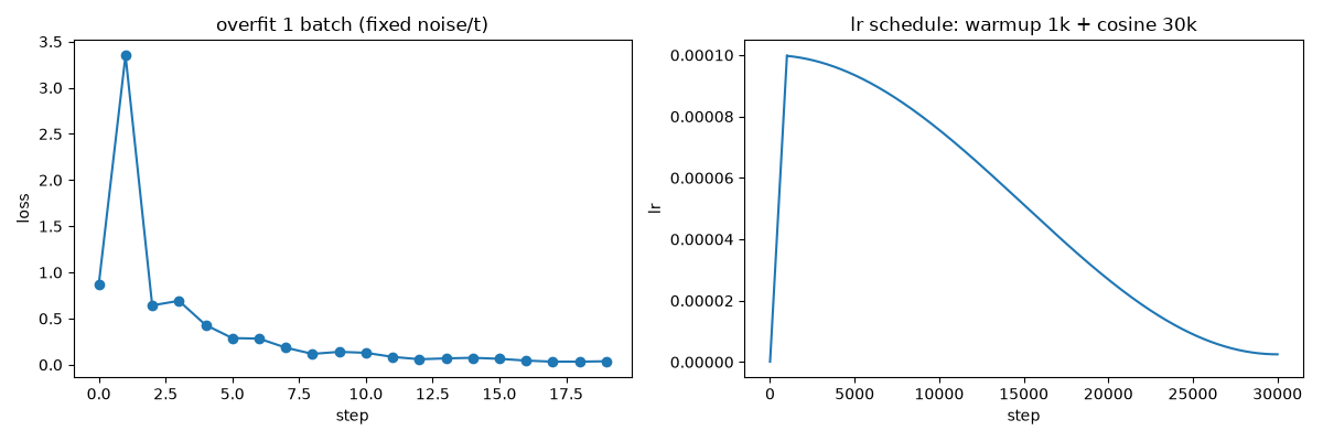
loss 가 0.87 → 0.04 로 떨어진다. (근데 이건 똑똑해진게 아니라 외운거다;;)

같은 batch 2개(문제 2개)를 20번 반복해서 푼거라, 기출 2문제만 달달 외운 학생이랑 같다. 그래도 “학습 루프가 고장없이 돈다” 는 확인한거다. (freeze W 도 안 변함)

step 1 에서 loss 가 3.35 로 튀는건 lr 1e-4 로 바로 시작해서다. Adam 은 첫 step 에 모든 파라메터를 lr 만큼 한꺼번에 움직이는데, 1억개가 동시에 확 움직이니까 흔들린다. 그래서 실제 학습은 lr 을 1e-7 부터 천천히 올린다 (warmup → cosine, 오른쪽 그래프 처럼).

Forward at the training

---

학습할때, forward에서 loss 값을 어떻게 구하는지 코드를 읽어보자. 눈여겨 봐야할 핵심 부분만 살펴보자.

• A: make_flow_matching_inputs → velocity(u_t) 와 noise (x_t) 를 시간에 따른 정답값을 추출
• B: Mask & Pad concat
• C: 1D → 2D attention Mask
• D: vlm_with_expert.forward with [prefix, suffix] both of them
• E: 받은 suffix → v_t 를 구하기
• F: Ground truth와 MSE 도출.

def forward(
        self, images, img_masks, lang_tokens, lang_masks, state, actions, noise=None, time=None
    ) -> Tensor:
        """Do a full training forward pass and compute the loss (batch_size x num_steps x num_motors)"""
        if noise is None:
            noise = self.sample_noise(actions.shape, actions.device)

        if time is None:
            time = self.sample_time(actions.shape[0], actions.device)

        # A: Flow matching got the ground truth (u_t)
        x_t, u_t, _ = make_flow_matching_inputs(actions, noise, time, convention=FlowConvention.NOISE_AT_ONE)
        prefix_embs, prefix_pad_masks, prefix_att_masks = self.embed_prefix(
            images, img_masks, lang_tokens, lang_masks, state=state
        )
        
        
        # B: Concat the mask and Pad (suffix + prefix)
        suffix_embs, suffix_pad_masks, suffix_att_masks = self.embed_suffix(x_t, time)

        pad_masks = torch.cat([prefix_pad_masks, suffix_pad_masks], dim=1)
        att_masks = torch.cat([prefix_att_masks, suffix_att_masks], dim=1)

        # C: 1D -> 2D mask w/ pad
        att_2d_masks = make_att_2d_masks(pad_masks, att_masks)
        position_ids = torch.cumsum(pad_masks, dim=1) - 1
        
        # D: Main Forward (attention)
        (_, suffix_out), _ = self.vlm_with_expert.forward(
            attention_mask=att_2d_masks,
            position_ids=position_ids,
            past_key_values=None,
            inputs_embeds=[prefix_embs, suffix_embs],
            use_cache=False,
        )
        
        # E: Suffix out -> velocity
        suffix_out = suffix_out[:, -self.config.chunk_size :]
        # Original openpi code, upcast attention output
        suffix_out = suffix_out.to(dtype=torch.float32)
        v_t = self.action_out_proj(suffix_out)
        
        # F: Get Loss
        losses = F.mse_loss(u_t, v_t, reduction="none")
        return losses

5. Fine-tuning preprocessing

---

4번은 batch 하나만 뽑아서 돌렸지만, 진짜 학습은 매 step 마다 새 batch 가 필요하다. 그리고 학습이 잘 됐는지 확인할 시험용 데이터도 따로 필요하다.

train / val 분리

영상(에피소드) 50개를 45개는 학습, 5개는 시험용으로 나눴다. 포인트는 frame 단위가 아니라 에피소드 단위로 나눈거다. frame 단위로 랜덤하게 나누면 같은 영상의 바로 옆 frame(1/30초 차이)이 train / val 에 섞여서, 기출문제 숫자만 바꿔서 시험 내는거랑 같아진다.

# total 50 Episodes or videos.
delta = {"action": [i / FPS for i in range(CHUNK)]}          # 미래 50 step 정답 chunk
TRAIN_EPS = list(range(0, 45))
VAL_EPS = list(range(45, 50))

DataLoader → 책갈피 꽂기 - iter()

Dataset 은 정돈된 창고라서 ds[230] 처럼 frame 1개씩만 꺼내준다. DataLoader 는 창고에서 랜덤으로 64개를 골라서 쟁반에 담아오는 직원. ([50, 6] x 64 → [64, 50, 6])

• num_workers=8 : 직원 8명이 GPU 가 학습하는 동안 다음 batch 들을 미리 디코딩해서 줄 세워둔다. GPU 는 한번에 batch 하나씩만 학습하지만 기다릴 필요가 없음
• iter() : 책갈피 꽂기. 이 순간 순서를 섞고 worker 들이 뜨기 시작한다

# Train Data Loader.
train_loader = DataLoader(train_ds, batch_size=args.batch_size, shuffle=True, drop_last=True,
                          num_workers=args.num_workers, pin_memory=DEVICE == "cuda",
                          persistent_workers=args.num_workers > 0)
train_iter = iter(train_loader)

next(train_iter): 책갈피 위치에서 다음 것 하나를 꺼내고 책갈피를 한 칸 옮기는 메서드

def next_batch():
    # 에폭 경계 없이 계속 batch 를 뽑기 (lerobot_train 도 이렇게 cycle 함)
    global train_iter
    try:
        return next(train_iter)
    except StopIteration:
        train_iter = iter(train_loader)                   # persistent worker 재사용
        return next(train_iter)

한 바퀴(약 165 batch) 다 돌면 StopIteration 이 뜨는데, 그때 다시 섞고 책갈피를 처음으로 옮긴다. 우리는 epoch 이 아니라 step 20,000 번 단위로 돌리니까 (약 120 바퀴) 끝나면 알아서 다시 시작하게 만든것.

실제 학습 루프에서는 이렇게 쓴다. 꺼낸 raw batch 를 바로 preprocessor 에 넣는다.

def prepare(raw):
    return pre(rename_batch_keys(dict(raw), RENAME))   # 카메라 이름 변경 → 정규화 / 토크나이즈 / GPU

for step in range(1, args.steps + 1):
    batch = prepare(next_batch())        # 창고에서 64개 꺼내기 → 손질
    ...

Evaluation (val)

학습 중에 처음 보는 에피소드(45~49)로 시험을 본다. 2가지다.

(1) val loss : 500 step 마다. 중요한건 val batch 와 noise / t 를 고정한거다.

(매번 랜덤이면 val loss 가 바뀐게 모델 때문인지 문제 때문인지 모름. 매번 같은 시험지로 보는것)

val_raw_batches = list(itertools.islice(val_loader, 4))   # 고정된 64 x 4 = 256 frame
val_batches = [prepare(b) for b in val_raw_batches]
# val 용 고정 noise / t
g = torch.Generator(device="cpu").manual_seed(123)
val_noise = [torch.randn(b[ACTION].shape[0], CHUNK, 32, generator=g).to(DEVICE) for b in val_batches]
val_time  = [(torch.rand(b[ACTION].shape[0], generator=g) * 0.999 + 0.001).to(DEVICE) for b in val_batches]

@torch.no_grad()
def val_loss():
    vals = [policy.forward(b, noise=n, time=t)[0].item() for b, n, t in zip(val_batches, val_noise, val_time)]
    return sum(vals) / len(vals)

(2) 실제 action 오차 (MAE) : loss 가 낮다고 로봇이 잘 움직이는건 아니다. 그래서 추론때랑 똑같이 10 step denoising 으로 action chunk 를 뽑고, 역정규화해서 정답이랑 도(°) 단위로 비교한다.

@torch.no_grad()
def predict_val(tag):
    policy.reset()                                      # action queue 비우기
    b = val_batches[0]
    pred = post(policy.predict_action_chunk(b))         # [B, 50, 6] 역정규화 (도 단위)
    gt = val_raw_batches[0][ACTION].to(pred.device)     # [B, 50, 6] 정답
    valid = ~b["action_is_pad"].to(pred.device)
    mae = ((pred - gt).abs() * valid[..., None]).sum(dim=(0, 1)) / valid.sum()   # 관절별 평균 오차
    policy.train()
    return pred[0].cpu(), gt[0].cpu(), mae.mean().item()

학습 전(base) 모델은 관절 평균 17.7도 틀렸다.

6. Fine-tuning result

---

이전에는 구조 확인용이었고, 이제 진짜로 GPU 빌려서 학습시켜보자. 바뀐건 다음과 같다:

• batch 2 → 64, step 20 → 20,000 (공식 세팅)
• 같은 batch 반복 → 매 step 새로운 랜덤 64개, noise / t 도 매번 랜덤
• lr 고정 → warmup + cosine scheduler 실제 적용
• train / val 분리: 에피소드 0~44 는 학습, 45~49 는 시험용 (학습에 한번도 안 보여줌)

TRAIN_EPS = list(range(0, 45))
VAL_EPS = list(range(45, 50))
train_ds = LeRobotDataset(..., episodes=TRAIN_EPS, delta_timestamps=delta)
val_ds = LeRobotDataset(..., episodes=VAL_EPS, delta_timestamps=delta)

#학습하는동안 learning rate를 자동으로 바꿔주는 장치.
scheduler = policy.config.get_scheduler_preset().build(optimizer, num_training_steps=args.steps)

# 학습 loop on.
for step in range(1, args.steps + 1):
    batch = prepare(next_batch())        # 매번 새 batch 64개
    optimizer.zero_grad()
    loss, _ = policy.forward(batch)      # noise / t 랜덤
    loss.backward()
    torch.nn.utils.clip_grad_norm_(policy.parameters(), 10)
    optimizer.step()
    scheduler.step()                     # lr 갱신 (4번엔 없던거)
    if step % 500 == 0:
        val_loss()                       # 처음 보는 에피소드로 시험

루프 자체는 4번이랑 똑같다. 그냥 문제집을 바꿔가면서 엄청 많이 돌린거다.

GPU

---

Mac CPU 로는 20 step 도 30분 넘게 걸려서 RunPod 에서 GPU 를 빌렸다.

• NVIDIA A40 (48GB), Secure Cloud, $0.59/hr
• 메모리 17GB 사용, 속도 1 it/s → 20,000 step 이면 약 5.4시간 (공식 문서 기준 A100 으로도 약 4시간)

Results

---

step	0	500	1500	2500	3500
val loss	0.938	0.279	0.267	0.284	0.361

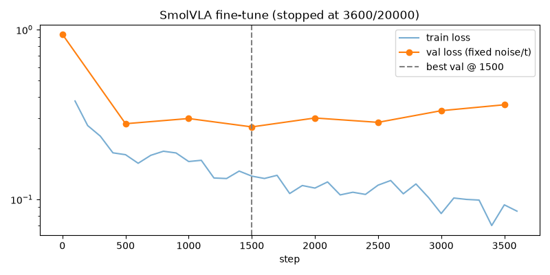
train loss 는 0.38 → 0.08 로 계속 떨어지는데, val loss 는 1500 step 에서 최저점 찍고 다시 올라간다. 이게 과적합(overfitting)이다. 기출문제만 계속 풀다보니 답을 외워버려서, 처음 보는 문제는 오히려 더 못푸는 상태. 그래서 3600 step 에서 그냥 멈췄다 ㅋㅋ (약 1시간)

공식 20,000 step 은 그냥 기본값이다. 이 데이터(에피소드 50개) 는 1500~2000 step 이면 충분했다. step 수는 감으로 정하는게 아니라 val loss 보고 정해야 한다.

Summary

---

일단 실제 데이터, 모델 , and gpu를 활용해서 실험을 진행한 것 자체에서 의미가 있다.

Train data 준비하기

---

• train 데이터 10,584 frame (에피소드 45개) → 모든 데이터 섞은 다음에 (64 = B)개씩 그룹화하고, B1, B2, …, B165 로 나열해준다. (10,584 = 64 x 165 + 24, 남는 24개는 버림 drop_last=True)
• 그리고 이제 그 1번부터 순서대로 학습에 사용하는 것이다. B165 까지 다 쓰면 다시 섞어서 새로운 B1 ~ B165 를 만든다. (매 바퀴 조합이 다름)
• 여기서 모든 학습한 배치의 갯수가 # of iteration (= step) 이고, epoch 는 모든 데이터를 한바퀴 돌면 1 epoch를 학습했다라고 부른다.
  • 1 epoch = 165 iteration
  • 공식 20,000 step = 약 121 epoch
  • 우리가 멈춘 3,600 step = 약 22 epoch, val loss 최저점 1,500 step = 약 9 epoch
• learning rate 를 dynamic하게 바꿀 수가 있다. (warmup → cosine scheduler, 처음엔 아주 작게 시작해서 올렸다가 천천히 내린다)

새로 배운 핵심들

---

• Freeze는 3단계다: config 스위치 → requires_grad = False → train() 에서 .eval() 고정. 그래서 전체 4.5억개 중 22.2%(약 1억개, 거의 action expert) 만 학습된다.
• 얼려도 gradient는 흐른다: requires_grad = False 는 그 가중치 업데이트만 막지, 그 층을 통과하는 역전파는 안 막는다. 그래서 얼어있는 VLM 뒤에 있는 state_proj 에도 grad 가 생긴다.
• 학습 forward는 추론이랑 다르다: 추론은 prefix를 KV cache로 만들고 denoise 10번을 돌지만, 학습은 [prefix, suffix] 를 한번에 넣고 랜덤 t 하나에서 velocity MSE 한번만 구한다. (10 step 안 돈다)
• 같은 batch로 loss가 떨어지는 건 외운것: 학습 루프가 고장 없이 도는지 확인하는 sanity check 용도일 뿐이다.
• train / val은 에피소드 단위로, val은 고정된 시험지로: frame 단위로 나누면 커닝이고, val batch / noise / t 를 고정해야 step 끼리 비교가 된다.
• loss만 보면 안된다: 실제로 denoising해서 뽑은 action을 도(°) 단위 MAE로도 봐야 로봇이 얼마나 틀리는지 알 수 있다. (base 모델 17.7도)
• step 수는 val loss가 정한다: 공식 20,000 step이 아니라, 이 데이터는 1,500 step(약 9 epoch)에서 val loss 최저 → 그 뒤로는 과적합이다.